Executive Summary
- Return profile: XLP earned 6.03% annualized with 10.61% volatility and a 13.57% maximum drawdown in the sample.
- Statistical edge: Weak. Variance-ratio tests do not reject a random-walk benchmark, and ARIMA selects (0,0,0), so daily return timing has not earned trust.
- Practical takeaway: Pivot from trying to predict tomorrow’s direction toward risk modeling, volatility targeting, relative strength, or explicitly backtested rules.
The conclusion is educational, not personalized financial advice. A trading strategy still needs explicit rule definitions, walk-forward validation, transaction costs, turnover, and benchmark comparisons.
Research Question
XLP is the defensive-allocation case. Consumer staples can be calmer than the market, but defensive behavior is not the same as a trading signal. The useful test is whether the ETF rewarded chasing strength, buying weakness, or simply managing exposure around risk. This note keeps the conclusion narrow: it forms a strategy hypothesis, not a live trading recommendation.
Analysis Date And Sample Window
Table 1. Analysis Date And Sample Window
| Field | Value |
|---|---|
| Publication date | 2026-06-01 |
| Analysis run date | 2026-06-02 |
| Sample window | 2023-01-03 to 2024-12-27 |
| Return observations | 499 |
| Data fetched | 2026-06-02 |
The sample window matters. Table 1 fixes the time period before any conclusion is drawn. The analysis uses the sample ending 2024-12-27, so the statistics should be read as evidence from that window rather than a claim about today’s market state.
Return Profile
Before testing any trading rule, we need the basic risk/reward map. Table 2 shows that XLP earned 6.03% annualized with 10.61% annualized volatility and a 13.57% maximum drawdown. The zero-rate Sharpe of 0.568 compares reward with realized volatility, which helps us judge whether the sample return compensated investors for the day-to-day risk.
Table 2. Return Profile
| Metric | Value |
|---|---|
| Annualized return | 6.03% |
| Annualized volatility | 10.61% |
| Zero-rate Sharpe | 0.568 |
| Max drawdown | 13.57% |
| Lag-1 autocorrelation | -0.051 |
What this means: The return and drawdown numbers set the risk/reward backdrop for XLP. The lag-1 autocorrelation of -0.051 leans negative, but it still needs confirmation before it can support a mean-reversion rule.
Distribution Diagnostics
The distribution check in Table 3 asks whether the daily returns look close to normal or whether unusual tails and asymmetry need to be taken seriously. This matters because many simple trading rules look cleaner when returns are assumed to be well-behaved.
Table 3. Distribution Diagnostics
| Test | Statistic | P_Value | Reject_Normality |
|---|---|---|---|
| Jarque-Bera | 10.1719 | 0.0062 | Yes ** |
| Anderson-Darling | 0.4267 | 0.3126 | No |
| Kolmogorov-Smirnov (normal) | 0.0276 | 0.8420 | No |
| Shapiro-Wilk | 0.9936 | 0.0328 | Yes ** |
What this means: Distribution tests ask whether daily returns behave like the clean bell curve assumed in many textbook models. 2 of the normality tests reject the normal-return benchmark. For XLP, this matters because non-normal returns can make a simple momentum or mean-reversion rule look calmer in a model than it feels in a real portfolio.
Momentum Versus Mean Reversion
The variance-ratio test in Table 4 asks whether returns behave like a random walk across different holding windows. Here, q is the return horizon in trading days, so q=4 is roughly one trading week. Quant researchers care because a value far from 1 can hint at momentum or mean reversion, but only the p-values tell us whether that hint is strong enough to trust. For XLP, VR q=2 is 0.952 with a bootstrap p-value of 0.278, q=4 is 0.864 with a p-value of 0.100, and q=16 is 0.933 with a p-value of 0.814. None of the reported horizons rejects the random-walk benchmark, so the market was too efficient at these short horizons for a simple daily trend-following or mean-reversion rule to stand on its own.
Table 4. Momentum Versus Mean Reversion
| Horizon | VR | HC_Statistic | Bootstrap_p | Reject_Random_Walk |
|---|---|---|---|---|
| VR q=2 | 0.952 | -1.115 | 0.278 | No |
| VR q=4 | 0.864 | -1.718 | 0.100 | No |
| VR q=8 | 0.867 | -1.066 | 0.324 | No |
| VR q=16 | 0.933 | -0.456 | 0.814 | No |
What this means: XLP’s recent return direction did not offer a reliable clue across the tested 2, 4, 8, and 16-day windows. That is the uncomfortable reality of liquid markets: price can move strongly over a sample, yet still give very little daily timing edge. A trader can still design rules, but the rules need to prove themselves in a backtest rather than leaning on this table.
Return Series Checks
The stationarity checks in Table 5 ask whether the return series is stable enough for time-series modeling. Quant researchers care because many models assume the return process does not drift like an unanchored price level. These tests support the mechanics of the research note; they do not create an investment edge by themselves.
Table 5. Return Series Checks
| Test | P_Value |
|---|---|
| ADF returns | 0.0100 |
| KPSS returns | 0.1000 |
| Phillips-Perron returns | 0.0100 |
Mean-Equation Model
The mean-equation model in Table 6 asks whether daily returns have a repeatable pattern after accounting for simple time-series structure. ARIMA is useful because it tests whether past returns help explain future returns in a formal model rather than by eye. The selected ARIMA order is (0,0,0), residual Ljung-Box p-value is 0.6422, and the ARFIMA median d estimate is 0.050. For XLP, that is not a strong case for a standalone return-timing model.
Table 6. Mean-Equation Model
| Metric | Value |
|---|---|
| ARIMA order | (0,0,0) |
| ARFIMA d median | 0.050 |
| Residual Ljung-Box p | 0.6422 |
| Squared-residual Ljung-Box p | 0.0092 |
| Model conclusion | short_memory |
What this means: The mean model did not find a useful daily return equation, which means the return process offered little memory for a simple forecasting rule. The squared-residual Ljung-Box p-value of 0.0092 checks whether large moves tend to cluster after the mean model. A low value means risk has memory even if direction does not, which explains why the analysis pivots from return timing to volatility modeling.
Volatility Context
The volatility evidence matters because weak return timing does not remove portfolio risk. The ARCH-effects result is weak_arch_effects, which makes risk controls a reasonable candidate for later testing.
Volatility Model Diagnostics
The volatility model in Table 7 shifts the question from direction to risk. Quants care about this because even when tomorrow’s return is hard to forecast, tomorrow’s volatility may be more predictable. That can support position sizing and stress testing, but it does not turn a weak return signal into a validated trading rule.
Table 7. Volatility Model Diagnostics
| Metric | Value |
|---|---|
| Best volatility model | sGARCH (norm) |
| Persistence | 0.998 |
| Half-life | 319.444 trading days |
| Squared standardized residual p | 0.0271 |
What this means: If a volatility shock hits XLP, the fitted model estimates a half-life of about 319.4 trading days. GARCH models are built for this problem: they estimate how volatility clusters and fades after shocks. In practical terms, if a market shock doubles the asset’s volatility, a portfolio manager would expect it to take roughly this long for risk to settle halfway back toward normal, which can dictate how long to reduce position sizes.
Regime Context
Regime analysis asks whether the asset behaved differently across market states. That matters because some strategies only work when volatility, trend, liquidity, or macro conditions are favorable. Here, the classification is stable with 0 detected structural breakpoints, so any regime filter remains a candidate to test rather than a conclusion from this article.
What this means: The regime label is context only. It can suggest a future conditional test, but it does not validate a regime strategy by itself.
Long-Memory Diagnostics
The long-memory check in Table 8 asks whether returns contain a slower persistence pattern that short-horizon tests can miss. This matters because a two-week variance-ratio test can look neutral even when a broader trend or reversal effect appears over longer horizons.
Table 8. Long-Memory Diagnostics
| Estimator | Estimate | Note |
|---|---|---|
| R/S (simple) | 0.554 | Hurst (1951) simple R/S |
| R/S (corrected) | 0.601 | Bias-corrected R/S |
| R/S (empirical) | 0.543 | Empirical aggregated R/S |
| Whittle (fGn) | n/a | Whittle MLE in frequency domain |
| GPH → H | 0.544 | d=0.0441, se=0.1364 |
| Sperio → H | 0.556 | d=0.0557, se=0.0570 |
What this means: Long-memory tests ask whether return behavior persists beyond the short windows in the variance-ratio table. Hurst values near 0.5 usually point to little memory, values above 0.5 lean toward persistence, and values below 0.5 lean toward mean reversion. For XLP, the median Hurst estimate is 0.554, with GPH d at 0.044 and Sperio d at 0.056. That keeps the interpretation cautious: any longer-horizon signal still needs to prove itself in a direct strategy test.
Rolling Risk Diagnostics
The rolling-risk view in Table 9 checks whether the full-sample averages hide changing risk conditions. Quant researchers care because a strategy that looks acceptable on average can still fail if volatility, drawdown pressure, or tail behavior shifts at the wrong time.
Table 9. Rolling Risk Diagnostics
| Metric | Current | Mean | Min | Max |
|---|---|---|---|---|
| Vol 21d (ann.) | 0.086 | 0.103 | 0.061 | 0.167 |
| Vol 63d (ann.) | 0.097 | 0.103 | 0.084 | 0.134 |
| Sharpe 252d | 1.298 | 0.949 | -0.135 | 2.344 |
| Sortino 252d | 1.339 | 0.959 | -0.128 | 2.420 |
| Calmar 252d | 2.466 | 1.557 | -0.112 | 5.612 |
| ExKurtosis 60d | -0.210 | -0.061 | -1.000 | 1.600 |
What this means: Rolling risk checks whether the asset’s risk profile is stable through time. The 63-day rolling volatility is 9.67% versus a sample mean of 10.29%. The 252-day rolling Sharpe is 1.298, which shows how the risk/reward profile looked near the sample end rather than across the full window only. The 60-day excess kurtosis is -0.210, a reminder that recent large moves can cluster even when average returns look orderly. For a trader, this supports testing position sizing and volatility controls before trusting a fixed-exposure rule.
Tail-Risk Diagnostics
The tail-risk check in Table 10 asks how severe the rare loss days were in the sample. This is useful for strategy design because a rule can have ordinary average returns and still be unacceptable if the left tail is too expensive to sit through.
Table 10. Tail-Risk Diagnostics
| Metric | Value |
|---|---|
| Threshold | 1.00% |
| Exceedances | 24 |
| EVT VaR 95% | 0.99% |
| EVT ES 95% | 1.37% |
| EVT VaR 99% | 1.58% |
| EVT ES 99% | 2.07% |
What this means: EVT focuses on the left tail: the rare loss days that can dominate a strategy’s real-world experience. For XLP, the 99% EVT loss estimate is 1.58% and the expected loss beyond that threshold is 2.07%, based on 24 exceedances. With a short daily sample this is a diagnostic, not a promise about future worst-case losses.
Distribution Fit Diagnostics
The distribution-fit comparison in Table 11 asks which probability model best describes the return shape. This matters because later backtests and risk estimates can be too optimistic if they assume normal returns when the data prefer a heavier-tailed model.
Table 11. Distribution Fit Diagnostics
| Model | Parameters | AIC | BIC | Delta_AIC |
|---|---|---|---|---|
| Student-t | 3 | -3579.876 | -3567.238 | 0.000 |
| Skew-t | 4 | -3579.013 | -3562.162 | 0.863 |
| NIG | 4 | -3578.573 | -3561.723 | 1.302 |
| Normal | 2 | -3578.543 | -3570.117 | 1.333 |
| VG | 4 | -3578.195 | -3561.344 | 1.681 |
What this means: Distribution fitting asks which return shape best matches the sample once normality looks too simple. For XLP, the best fit is Student-t. The second-best model is only 0.863 AIC points behind, so the ranking should be read as close rather than decisive. This helps set risk assumptions for later backtests; it does not create a return-timing edge by itself.
Drawdown Diagnostics
The drawdown review in Table 12 checks the realized downside path behind the strategy hypothesis. This is where a good-looking average return is forced to answer a harder question: how much pain did the investor have to sit through?
Table 12. Drawdown Diagnostics
| Metric | Value | Note | ||
|---|---|---|---|---|
| Max Drawdown | -13.37% | Trough on 2023-10-12 | ||
| Calmar Ratio | 0.451 | Weak (<0.5) | ||
| Sharpe Ratio (ann.) | 0.568 | Good | ||
| Sortino Ratio | 0.564 | — | ||
| Ann. Volatility | 10.61% | — | ||
| #1 2023-05-02 | -13.37% | Trough 2023-10-12 | Length 114d | Recovery 103d |
| #2 2023-01-09 | -6.16% | Trough 2023-03-10 | Length 43d | Recovery 21d |
| #3 2024-09-17 | -5.13% | Trough 2024-12-23 | Length 69d | Recovery Ongoingd |
What this means: Drawdown analysis asks how much capital pain the sample required, not just how attractive the average return looked. For XLP, the maximum drawdown was 13.37%, with a Calmar ratio of 0.451 and a Sharpe ratio of 0.568. That is useful because a strategy hypothesis has to survive the bad stretches, not only the full-sample average.
Visual Evidence
The charts below come from the same statistical evidence used in the article. They are included to make the risk path easier to inspect, not to add a separate signal.
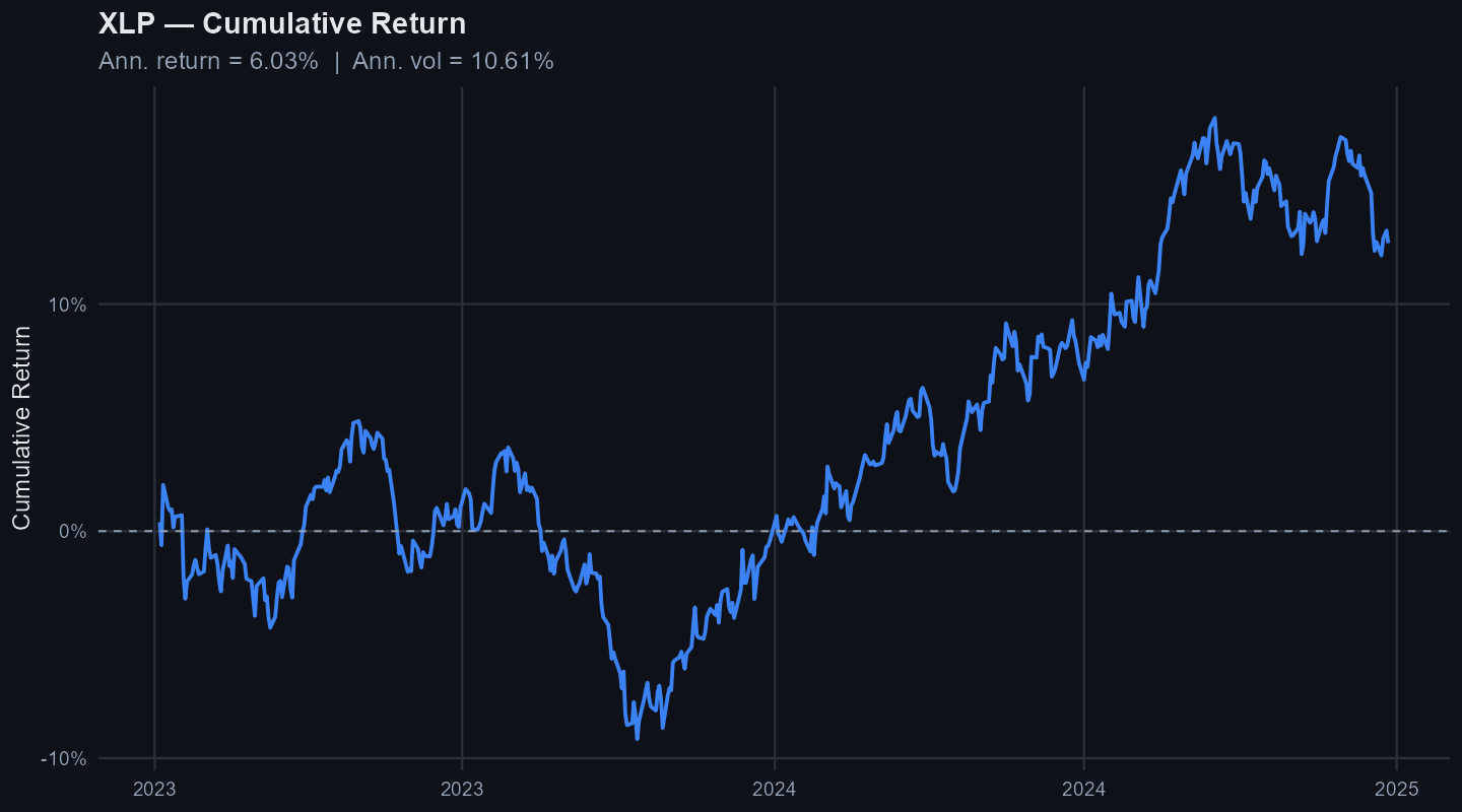
Cumulative return shows the path an investor actually had to sit through.
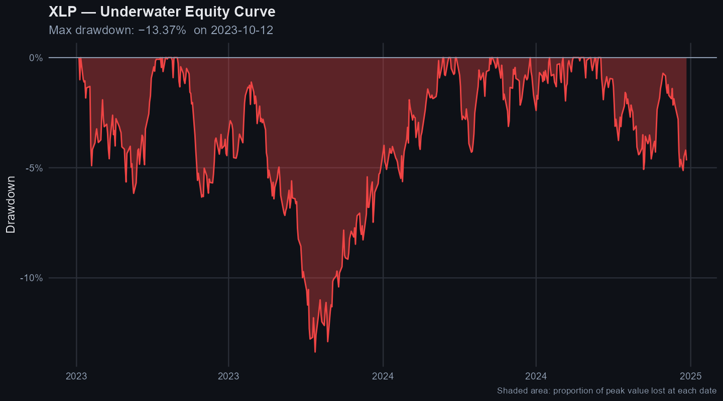
Drawdown makes the downside periods visible instead of hiding them inside one full-sample return number.
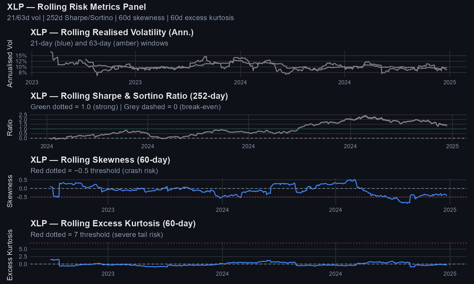
Rolling risk checks whether volatility and risk-adjusted returns were stable or clustered in specific periods.
Candidate Strategy Hypothesis
For XLP, the practical hypothesis is defensive. If the return signal is weak, the next design should ask whether volatility controls, drawdown limits, or market-regime filters improve the allocation profile without pretending that daily timing has been proven. The volatility evidence also matters: clustered variance means position sizing may be more useful than trying to forecast the next daily return.
The next tests that would add the most value are:
- Longer-horizon momentum tests, because the 2 to 16-day windows may be too short for the way many equity trends develop.
- Benchmark-relative momentum, because an asset can fail as a standalone timing trade but still matter in a pairs, sector-rotation, or relative-strength framework.
- Walk-forward rule tests with transaction costs, turnover, and cash or benchmark comparisons.
For automated research workflows, the resulting strategy hypothesis can be represented as:
{
  "strategy_name": "XLP Risk-Aware Allocation Test",
  "strategy_status": "hypothesis_for_backtest",
  "strategy_type": "risk_managed_allocation",
  "asset": "XLP",
  "core_thesis": "For XLP, the practical hypothesis is defensive. If the return signal is weak, the next design should ask whether volatility controls, drawdown limits, or market-regime filters improve the allocation profile without pretending that daily timing has been proven. The volatility evidence also matters: clustered variance means position sizing may be more useful than trying to forecast the next daily return.",
  "required_backtests": ["walk-forward validation", "buy-and-hold asset benchmark", "broad market benchmark", "cash or T-bill benchmark", "transaction costs", "turnover"],
  "not_investment_advice": true
}
What Would Change My Mind?
A good strategy-selection note should be falsifiable. These are the findings that would make the hypothesis stronger or force a different conclusion:
- Variance-ratio results would need to reject the random-walk benchmark at the relevant holding horizons, with p-values strong enough to survive a skeptical read.
- The mean-equation model would need to find useful structure in returns rather than selecting a flat mean process or leaving only noise in the residuals.
- A walk-forward backtest would need to beat buy-and-hold, cash or T-bills, and the relevant benchmark after transaction costs and turnover.
- Risk-managed variants would need to improve drawdown, volatility, or risk-adjusted return without simply hiding risk through lower exposure.
- For XLP, a defensive allocation rule would need to reduce drawdowns or portfolio volatility while keeping enough return participation to justify the complexity.
Backtested Results
The downloadable backtested results are planned for a later implementation step. They should include walk-forward results, benchmarks, turnover, and transaction-cost sensitivity before any rule is treated as validated.
Limitations
This article is a preliminary strategy-selection note for the 2023-01-03 to 2024-12-27 sample. It is useful for deciding what to test next; it is not a production trading rule.