Executive Summary
- Return profile: SPY earned 23.94% annualized with 12.81% volatility and a 10.15% maximum drawdown in the sample.
- Statistical edge: Weak. Variance-ratio tests do not reject a random-walk benchmark, and ARIMA selects (0,0,0), so daily return timing has not earned trust.
- Practical takeaway: Pivot from trying to predict tomorrow’s direction toward risk modeling, volatility targeting, relative strength, or explicitly backtested rules.
The conclusion is educational, not personalized financial advice. A trading strategy still needs explicit rule definitions, walk-forward validation, transaction costs, turnover, and benchmark comparisons.
Research Question
SPY is the broad-market efficiency test. When an asset is this liquid and this widely watched, simple daily patterns often disappear quickly. The useful question is whether the 23.94% annualized return and 12.81% volatility point toward a timing rule, or toward portfolio-level risk budgeting. This note keeps the conclusion narrow: it forms a strategy hypothesis, not a live trading recommendation.
Analysis Date And Sample Window
Table 1. Analysis Date And Sample Window
| Field | Value |
|---|---|
| Publication date | 2026-06-01 |
| Analysis run date | 2026-06-02 |
| Sample window | 2023-01-03 to 2024-12-27 |
| Return observations | 499 |
| Data fetched | 2026-06-01 |
The sample window matters. Table 1 fixes the time period before any conclusion is drawn. The analysis uses the sample ending 2024-12-27, so the statistics should be read as evidence from that window rather than a claim about today’s market state.
Return Profile
Before testing any trading rule, we need the basic risk/reward map. Table 2 shows that SPY earned 23.94% annualized with 12.81% annualized volatility and a 10.15% maximum drawdown. The zero-rate Sharpe of 1.869 compares reward with realized volatility, which helps us judge whether the sample return compensated investors for the day-to-day risk.
Table 2. Return Profile
| Metric | Value |
|---|---|
| Annualized return | 23.94% |
| Annualized volatility | 12.81% |
| Zero-rate Sharpe | 1.869 |
| Max drawdown | 10.15% |
| Lag-1 autocorrelation | 0.035 |
What this means: The return and drawdown numbers set the risk/reward backdrop for SPY. We also check lag-1 autocorrelation, which measures whether yesterday’s return carries memory into today’s return. The value of 0.035 is tiny, so yesterday’s price action gives very little help with today’s direction.
Distribution Diagnostics
The distribution check in Table 3 asks whether the daily returns look close to normal or whether unusual tails and asymmetry need to be taken seriously. This matters because many simple trading rules look cleaner when returns are assumed to be well-behaved.
Table 3. Distribution Diagnostics
| Test | Statistic | P_Value | Reject_Normality |
|---|---|---|---|
| Jarque-Bera | 19.8271 | < 0.001 | Yes ** |
| Anderson-Darling | 1.6447 | < 0.001 | Yes ** |
| Kolmogorov-Smirnov (normal) | 0.0568 | 0.0800 | No |
| Shapiro-Wilk | 0.9888 | < 0.001 | Yes ** |
What this means: Distribution tests ask whether daily returns behave like the clean bell curve assumed in many textbook models. 3 of the normality tests reject the normal-return benchmark. For SPY, this matters because non-normal returns can make a simple momentum or mean-reversion rule look calmer in a model than it feels in a real portfolio.
Momentum Versus Mean Reversion
The variance-ratio test in Table 4 asks whether returns behave like a random walk across different holding windows. Here, q is the return horizon in trading days, so q=4 is roughly one trading week. Quant researchers care because a value far from 1 can hint at momentum or mean reversion, but only the p-values tell us whether that hint is strong enough to trust. For SPY, VR q=2 is 1.034 with a bootstrap p-value of 0.480, q=4 is 0.986 with a p-value of 0.896, and q=16 is 0.829 with a p-value of 0.452. None of the reported horizons rejects the random-walk benchmark, so the market was too efficient at these short horizons for a simple daily trend-following or mean-reversion rule to stand on its own.
Table 4. Momentum Versus Mean Reversion
| Horizon | VR | HC_Statistic | Bootstrap_p | Reject_Random_Walk |
|---|---|---|---|---|
| VR q=2 | 1.034 | 0.680 | 0.480 | No |
| VR q=4 | 0.986 | -0.180 | 0.896 | No |
| VR q=8 | 0.902 | -0.792 | 0.500 | No |
| VR q=16 | 0.829 | -0.931 | 0.452 | No |
What this means: SPY’s recent return direction did not offer a reliable clue across the tested 2, 4, 8, and 16-day windows. That is the uncomfortable reality of liquid markets: price can move strongly over a sample, yet still give very little daily timing edge. A trader can still design rules, but the rules need to prove themselves in a backtest rather than leaning on this table.
Return Series Checks
The stationarity checks in Table 5 ask whether the return series is stable enough for time-series modeling. Quant researchers care because many models assume the return process does not drift like an unanchored price level. These tests support the mechanics of the research note; they do not create an investment edge by themselves.
Table 5. Return Series Checks
| Test | P_Value |
|---|---|
| ADF returns | 0.0100 |
| KPSS returns | 0.1000 |
| Phillips-Perron returns | 0.0100 |
Mean-Equation Model
The mean-equation model in Table 6 asks whether daily returns have a repeatable pattern after accounting for simple time-series structure. ARIMA is useful because it tests whether past returns help explain future returns in a formal model rather than by eye. The selected ARIMA order is (0,0,0), residual Ljung-Box p-value is 0.7782, and the ARFIMA median d estimate is -0.299. For SPY, that is not a strong case for a standalone return-timing model.
Table 6. Mean-Equation Model
| Metric | Value |
|---|---|
| ARIMA order | (0,0,0) |
| ARFIMA d median | -0.299 |
| Residual Ljung-Box p | 0.7782 |
| Squared-residual Ljung-Box p | 0.0004 |
| Model conclusion | anti_persistent |
What this means: The mean model did not find a useful daily return equation, which means the return process offered little memory for a simple forecasting rule. ARFIMA’s fractional d estimate looks for longer-memory behavior that a basic ARIMA model can miss. The negative value of -0.299 hints at anti-persistence, but the variance-ratio p-values decide whether that hint is strong enough to trade. The squared-residual Ljung-Box p-value of 0.0004 checks whether large moves tend to cluster after the mean model. A low value means risk has memory even if direction does not, which explains why the analysis pivots from return timing to volatility modeling.
Volatility Model Diagnostics
The volatility model in Table 7 shifts the question from direction to risk. Quants care about this because even when tomorrow’s return is hard to forecast, tomorrow’s volatility may be more predictable. That can support position sizing and stress testing, but it does not turn a weak return signal into a validated trading rule.
Table 7. Volatility Model Diagnostics
| Metric | Value |
|---|---|
| Best volatility model | eGARCH (sstd) |
| Persistence | 0.912 |
| Half-life | 7.517 trading days |
| Squared standardized residual p | 0.9241 |
What this means: If a volatility shock hits SPY, the fitted model estimates a half-life of about 7.5 trading days. GARCH models are built for this problem: they estimate how volatility clusters and fades after shocks. In practical terms, if a market shock doubles the asset’s volatility, a portfolio manager would expect it to take roughly this long for risk to settle halfway back toward normal, which can dictate how long to reduce position sizes.
Visual Evidence
The charts below come from the same statistical evidence used in the article. They are included to make the risk path easier to inspect, not to add a separate signal.
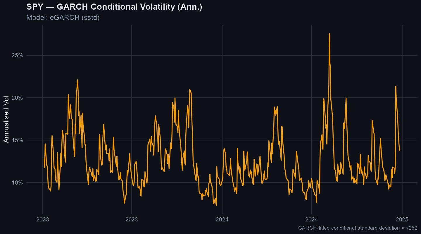
Conditional volatility shows whether risk came in bursts that a position-sizing rule would need to respect.
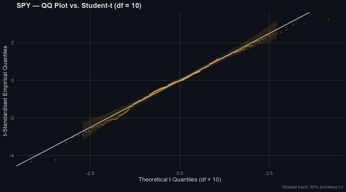
The tail-shape chart checks whether a simple normal-return assumption is too neat for the actual sample.
Candidate Strategy Hypothesis
For SPY, the practical hypothesis should start with efficiency. A broad index can reward long-run exposure while still offering little daily return predictability, so the next design should focus on volatility targeting, benchmark comparisons, and clean walk-forward rules. The volatility evidence also matters: clustered variance means position sizing may be more useful than trying to forecast the next daily return.
The next tests that would add the most value are:
- Longer-horizon momentum tests, because the 2 to 16-day windows may be too short for the way many equity trends develop.
- Benchmark-relative momentum, because an asset can fail as a standalone timing trade but still matter in a pairs, sector-rotation, or relative-strength framework.
- Walk-forward rule tests with transaction costs, turnover, and cash or benchmark comparisons.
- Overnight versus intraday return splits, because broad-market index behavior can differ sharply across those two return streams.
- Volatility-risk-premium tests that compare forecast volatility with implied volatility.
For automated research workflows, the resulting strategy hypothesis can be represented as:
{
  "strategy_name": "SPY Risk-Aware Allocation Test",
  "strategy_status": "hypothesis_for_backtest",
  "strategy_type": "risk_managed_allocation",
  "asset": "SPY",
  "core_thesis": "For SPY, the practical hypothesis should start with efficiency. A broad index can reward long-run exposure while still offering little daily return predictability, so the next design should focus on volatility targeting, benchmark comparisons, and clean walk-forward rules. The volatility evidence also matters: clustered variance means position sizing may be more useful than trying to forecast the next daily return.",
  "required_backtests": ["walk-forward validation", "buy-and-hold asset benchmark", "broad market benchmark", "cash or T-bill benchmark", "transaction costs", "turnover"],
  "not_investment_advice": true
}
What Would Change My Mind?
A good strategy-selection note should be falsifiable. These are the findings that would make the hypothesis stronger or force a different conclusion:
- Variance-ratio results would need to reject the random-walk benchmark at the relevant holding horizons, with p-values strong enough to survive a skeptical read.
- The mean-equation model would need to find useful structure in returns rather than selecting a flat mean process or leaving only noise in the residuals.
- A walk-forward backtest would need to beat buy-and-hold, cash or T-bills, and the relevant benchmark after transaction costs and turnover.
- Risk-managed variants would need to improve drawdown, volatility, or risk-adjusted return without simply hiding risk through lower exposure.
- For SPY, overnight versus intraday splits or volatility-risk-premium tests would need to show a cleaner source of edge than daily close-to-close direction.
Backtested Results
The downloadable backtested results are planned for a later implementation step. They should include walk-forward results, benchmarks, turnover, and transaction-cost sensitivity before any rule is treated as validated.
Limitations
This article is a preliminary strategy-selection note for the 2023-01-03 to 2024-12-27 sample. It is useful for deciding what to test next; it is not a production trading rule.