Can Google’s TabFM Predict Polymarket Crypto Markets? A Zero-Shot Backtest
Markets tested: Polymarket 5-minute BTC/ETH/XRP directional contracts | Sample: 1,320 walk-forward predictions across 55 folds | Models: TabFM (zero-shot), XGBoost, Random Forest, Logistic Regression, SVM
Executive Summary
Polymarket’s 5-minute crypto contracts ask a deceptively simple question — will price be higher or lower five minutes from now — and settle it fast enough that there is nowhere to hide a bad model. This report tests whether Google Research’s TabFM (Tabular Foundation Model) can compete with trained classifiers on that question, using a strict, leakage-free walk-forward framework across 1,320 prediction points on BTC, ETH, and XRP.
The headline result: TabFM’s zero-shot predictions — no training, no gradient updates, no hyperparameter search — hit 53.86% accuracy on XRP, edging out a fully trained XGBoost baseline (51.97%) on that asset and landing within a point of the best model on every symbol tested. A companion analysis of Logistic Regression coefficients, Random Forest importances, and SHAP values across all three assets converges on the same three drivers of these markets: short-term momentum, medium-term trend exhaustion, and intra-session mean reversion around VWAP.
1. The Prediction Challenge & Data Alignment
Polymarket’s 5-minute prediction markets for major cryptocurrencies (BTC, ETH, and XRP) resolve UP if price rises over the interval, and DOWN if it falls or stays flat.
Predicting these markets requires a strict, leakage-free data pipeline. For a market spanning 16:00 to 16:05:
- Predictions must be made at or before the
16:00start time. - Features must use technical indicators calculated strictly from historical data before
16:00. - This setup matches the operational constraint of entering a live trade right as the market opens.
This analysis uses a 2-week historical dataset (early April 2026), yielding approximately 1,445 closed markets per asset. Features are extracted across three timescales:
- Micro-scale (1-min): 5-minute rolling window statistics (mean, std, delta, last) of prices, session VWAP, and short-term RSI.
- Medium-scale (15-min and 1-hour): Standard indicators such as RSI, MACD, ADX, and Bollinger Bands.
- Macro-scale (1-day): Long-term trends such as the daily 200-day Simple Moving Average.
2. Foundation Models for Tabular Data: TabFM vs. Text LLMs
Traditional tabular machine learning models require explicit training by updating weights on a specific dataset. In contrast, TabFM is a Tabular Foundation Model that performs zero-shot classification.
Architecture and Inference Model
- Specialized Architecture: Unlike text-based LLMs (e.g., GPT-4 or Llama) that process character tokens and output natural language, TabFM is designed specifically for numerical and categorical tabular data. It maps columns to vector embeddings and outputs class probabilities directly.
- In-Context Learning (ICL): At inference time, TabFM’s weights remain frozen. Instead of parameter training, it reads a historical training set as "context" and makes predictions on test samples in a single forward pass, leveraging row and column attention mechanisms.
- Local Execution: The model runs entirely locally using PyTorch (
google/tabfm-1.0.0-pytorch) without external API calls or external text-generation servers.
3. Walk-Forward Backtesting: Folds & Runtime
Models are evaluated using sequential walk-forward validation, which models a real-world trading setup by expanding the training history over time.
Understanding Walk-Forward Folds
A "fold" represents a single backtesting step. For each fold:
- The model is presented with a historical training context (120 observations, representing 10 hours of market history).
- The model predicts the outcomes of the next test block (24 observations, representing a 2-hour window).
- The training window then expands by 24 observations, and the process repeats for the next fold.
- Across the 2-week dataset, this yields 55 sequential folds.
TabFM Computational Overhead
TabFM requires 7.5 to 8.5 seconds per fold, totaling approximately 7.5 minutes of compute time per asset (22 minutes total for BTC, ETH, and XRP combined).
Unlike traditional models that evaluate simple tree splits or linear equations in milliseconds, TabFM must pass the entire historical context window (120 rows) and the test queries together through a 24-block causal transformer network. On each step, the transformer dynamically calculates row-to-row and column-to-column attention weights, resulting in higher computational latency.
4. Performance Comparison
The table below outlines the backtesting accuracies and F1-scores across 1,320 prediction points:
| Symbol | Metric | Logistic Regression | Random Forest | Support Vector Machine (SVM) | XGBoost Baseline | TabFM (Zero-Shot) |
|---|---|---|---|---|---|---|
| BTC | Accuracy | 52.58% | 50.98% | 49.24% | 53.86% | 50.00% |
| F1-Score | 48.77% | 50.87% | 50.59% | 51.78% | 46.34% | |
| ETH | Accuracy | 50.98% | 51.82% | 53.86% | 53.11% | 51.06% |
| F1-Score | 43.59% | 47.18% | 45.87% | 49.47% | 41.27% | |
| XRP | Accuracy | 53.41% | 54.09% | 51.21% | 51.97% | 53.86% |
| F1-Score | 44.34% | 44.10% | 43.51% | 46.90% | 45.18% | |
| Overall | Accuracy | 52.32% | 52.30% | 51.44% | 52.98% | 51.64% |
| F1-Score | 45.57% | 47.38% | 46.66% | 49.43% | 44.35% |
TabFM’s zero-shot inference is highly competitive: it outperforms the trained XGBoost baseline on XRP (53.86% vs. 51.97%) and matches the top SVM accuracy on ETH — without ever seeing a labeled training example specific to this dataset.
5. Economic & Quantitative Interpretation of the Models
Analyzing the inner workings of Logistic Regression and Random Forest models reveals the structural dynamics of prediction market behavior.
5.1 Logistic Regression Coefficients: A Quantitative Rationale
The coefficients from the Logistic Regression models represent the change in log-odds of a market resolving UP for a one standard deviation increase in the corresponding feature.
| BTC Coefficients | ETH Coefficients | XRP Coefficients |
|---|---|---|
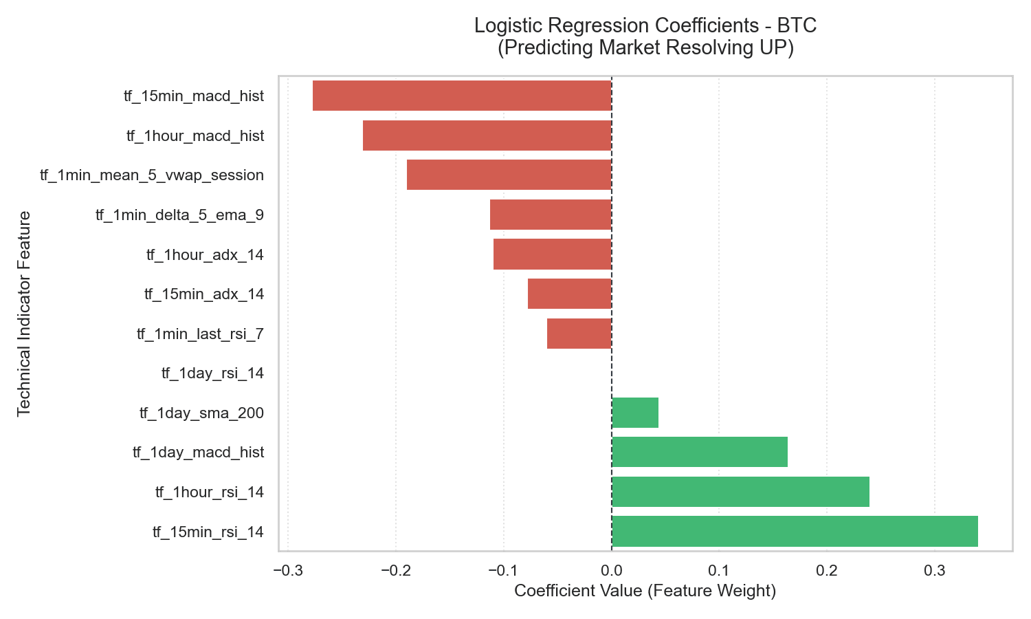 | 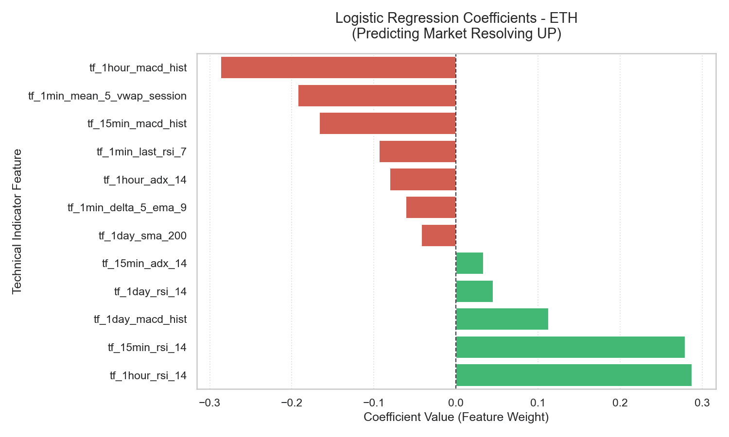 | 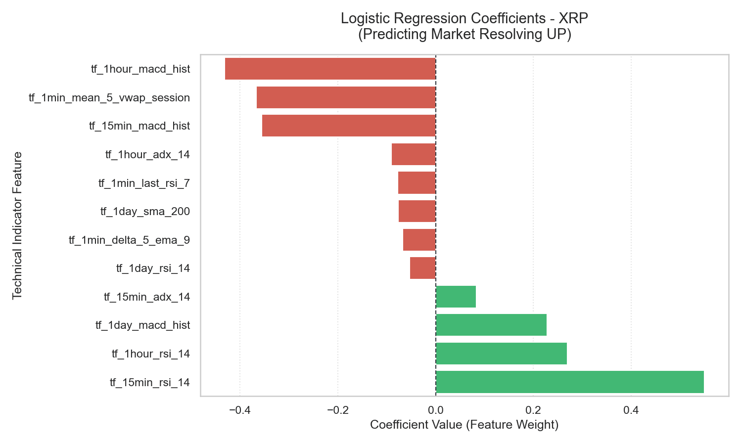 |
These charts show a highly consistent structure across all three assets:
- Momentum (
tf_15min_rsi_14) — Strongly Positive (e.g., +0.550 for XRP): Strong price momentum leading up to the market opening is the single strongest indicator of an UP resolution. Economically, this reflects short-term trend persistence — buying interest on a 15-minute horizon tends to carry over into the subsequent 5-minute window. - Trend Exhaustion (
tf_1hour_macd_hist) — Strongly Negative (e.g., -0.432 for XRP): The MACD histogram measures the acceleration of price trends. A highly elevated MACD histogram indicates the trend is moving at maximum velocity, which historically represents late-stage exhaustion. On a 5-minute horizon, these overextended trends are highly prone to reverse or consolidate. - Mean Reversion (
tf_1min_mean_5_vwap_session) — Strongly Negative (e.g., -0.367 for XRP): When price trades significantly above the session’s Volume-Weighted Average Price (VWAP) in the final 5 minutes, the probability of an UP resolution falls. This is intra-session mean reversion — liquidity providers and arbitrageurs fade extreme short-term price deviations back toward the average session value.
5.2 Random Forest Feature Importances
The Gini importances of the Random Forest model confirm the importance of these same variables.
| BTC RF Importances | ETH RF Importances | XRP RF Importances |
|---|---|---|
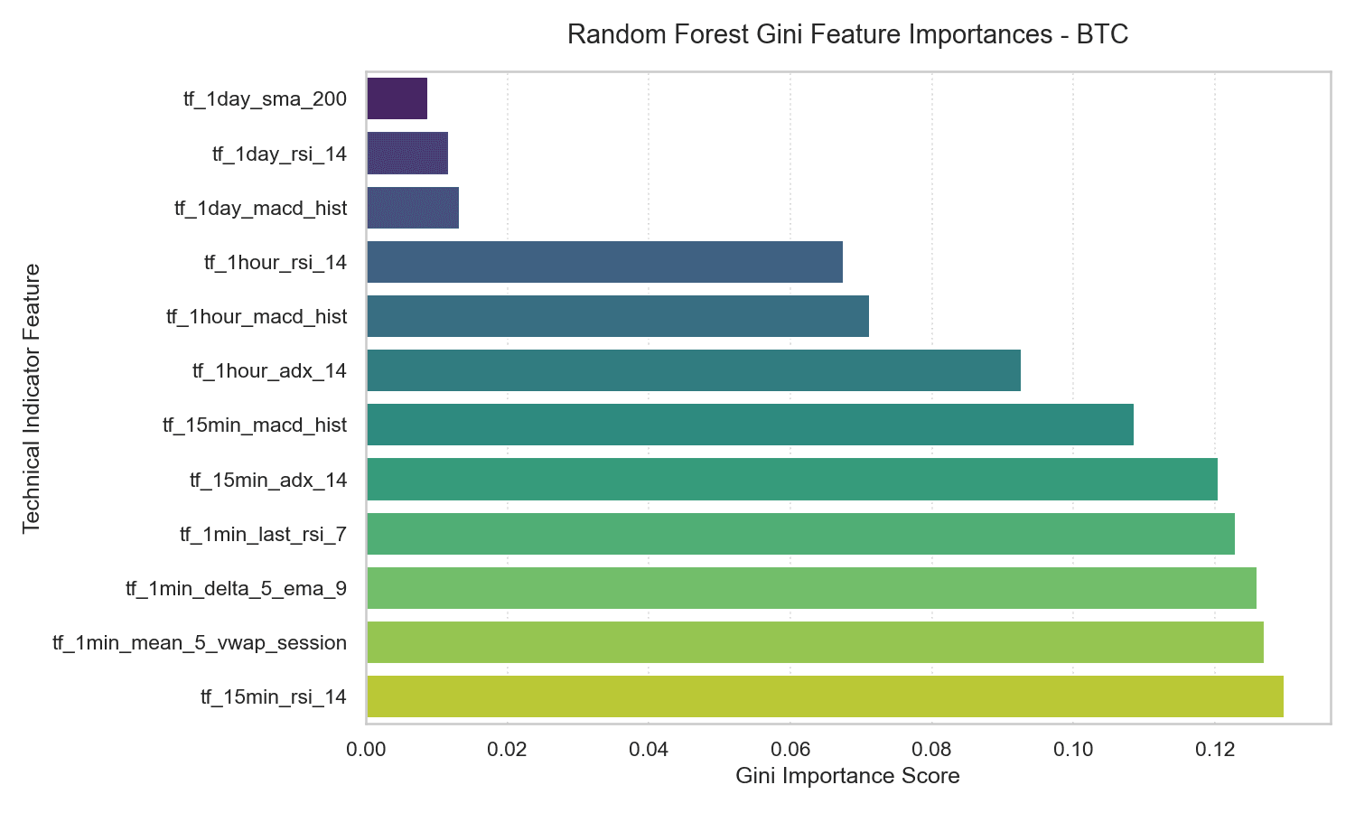 | 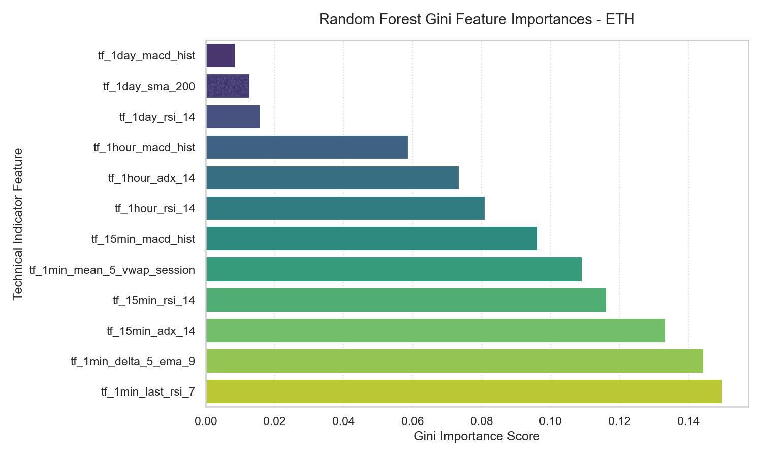 | 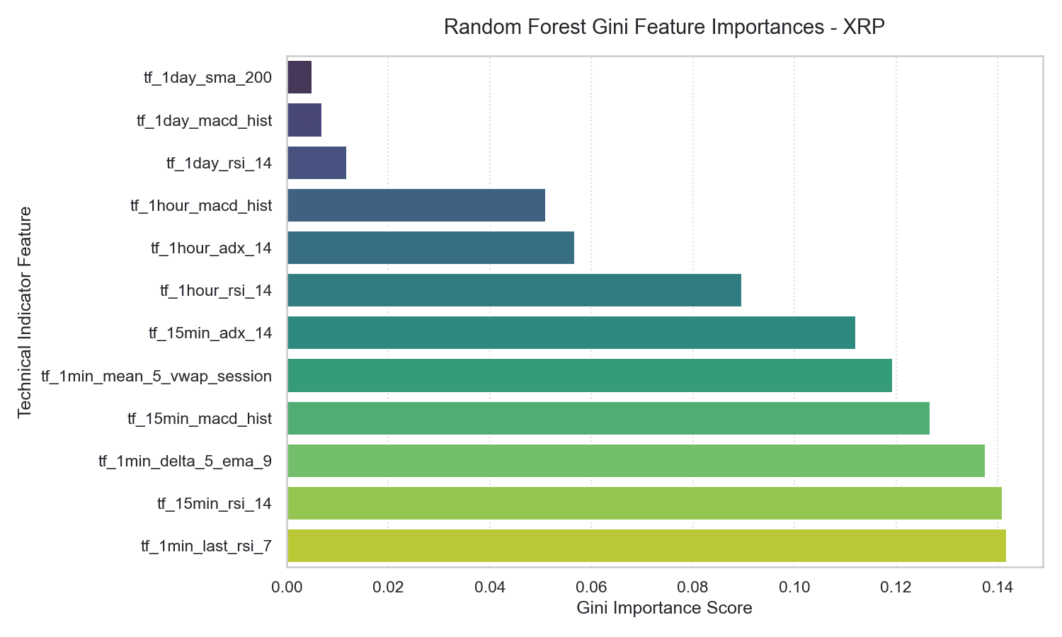 |
Short-term momentum (tf_15min_rsi_14) and session VWAP deviation (tf_1min_mean_5_vwap_session) dominate the importance scores, each accounting for 12% to 15% of the total predictive power. Conversely, long-term trends like the daily 200-day moving average (tf_1day_sma_200) account for less than 1% of the model’s split decisions — macro structural trends have essentially no statistical influence on 5-minute prediction horizons.
5.3 SHAP Summary (Beeswarm Analysis)
We computed Shapley Additive exPlanations (SHAP) values for the Random Forest model to analyze the non-linear relationship and direction of feature impact on individual predictions.
| BTC SHAP Summary | ETH SHAP Summary | XRP SHAP Summary |
|---|---|---|
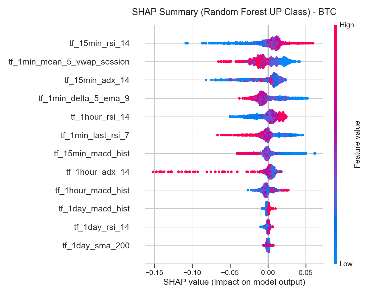 | 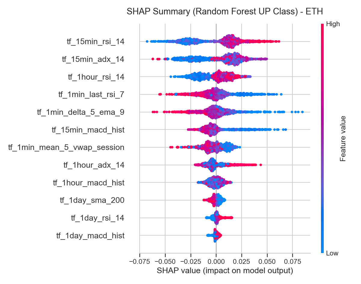 | 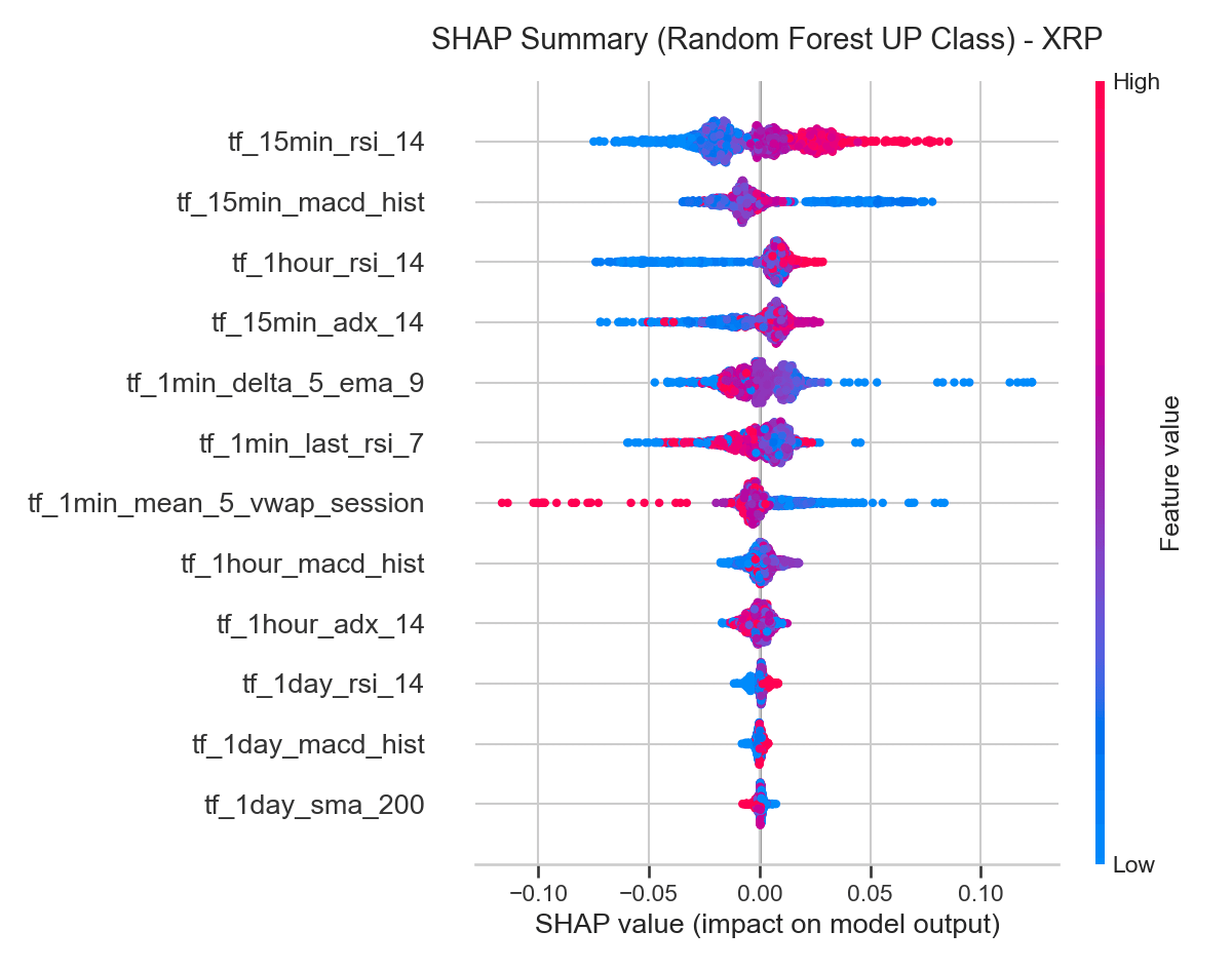 |
On a SHAP summary plot, horizontal position represents a feature’s impact on the model output (positive values increase the probability of an UP prediction), and color represents the feature value (red is high, blue is low):
tf_15min_rsi_14: Red dots cluster on the positive side of the SHAP axis, blue dots on the negative side — high RSI values consistently push predictions toward UP, a clean momentum effect.tf_1min_mean_5_vwap_session: Red dots cluster on the negative side, blue dots on the positive side — high deviations above the session VWAP push predictions toward DOWN, validating the mean-reversion driver.tf_1min_delta_5_ema_9: This variable measures trend acceleration over the final minutes. High values (red) associate with positive SHAP values, showing short-term trend acceleration acts as a reinforcing signal.
The alignment across Logistic Regression coefficients, Random Forest importances, and SHAP distributions confirms that both linear and non-linear models capture the same underlying market structure: following medium-term momentum, but fading extreme short-term deviations from the session average.
6. Correlation Analysis & Decoupling
The heatmap visualizes the correlation matrix of the key indicators.
| BTC Correlation Heatmap | ETH Correlation Heatmap | XRP Correlation Heatmap |
|---|---|---|
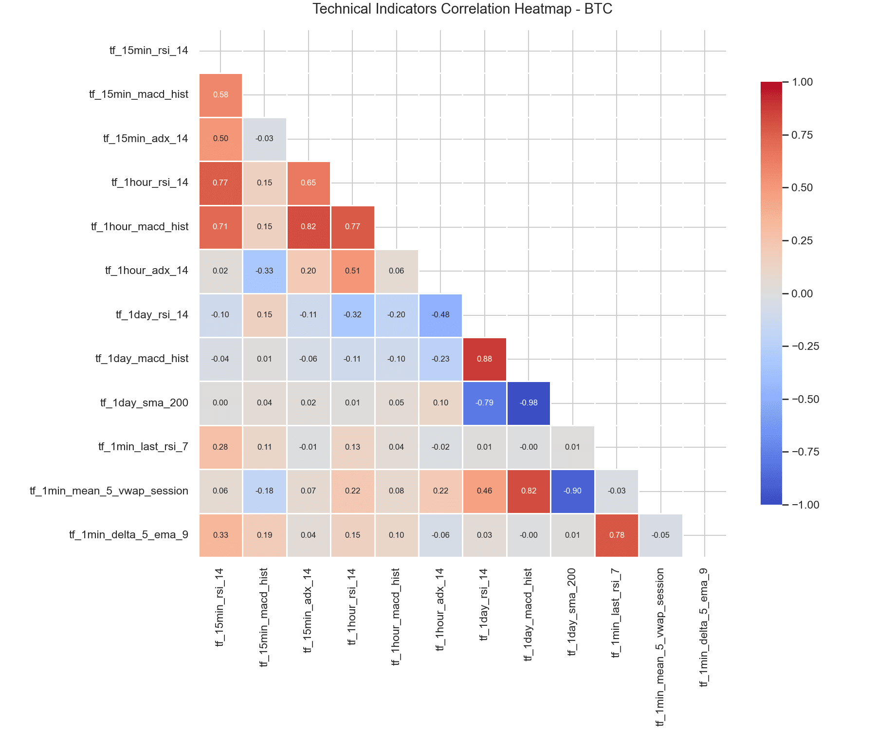 | 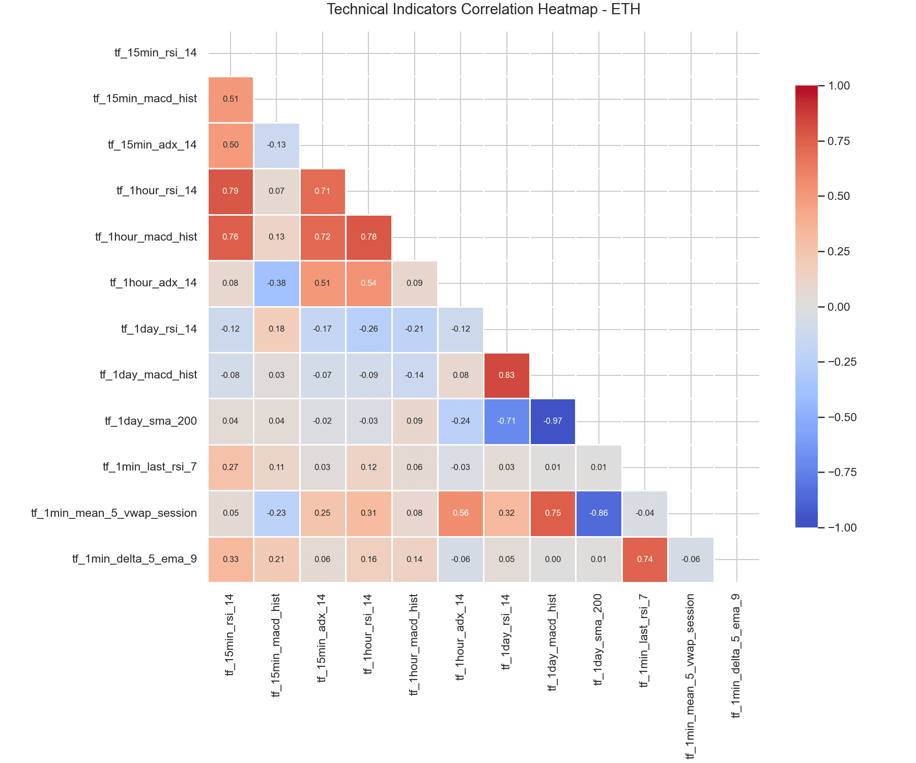 | 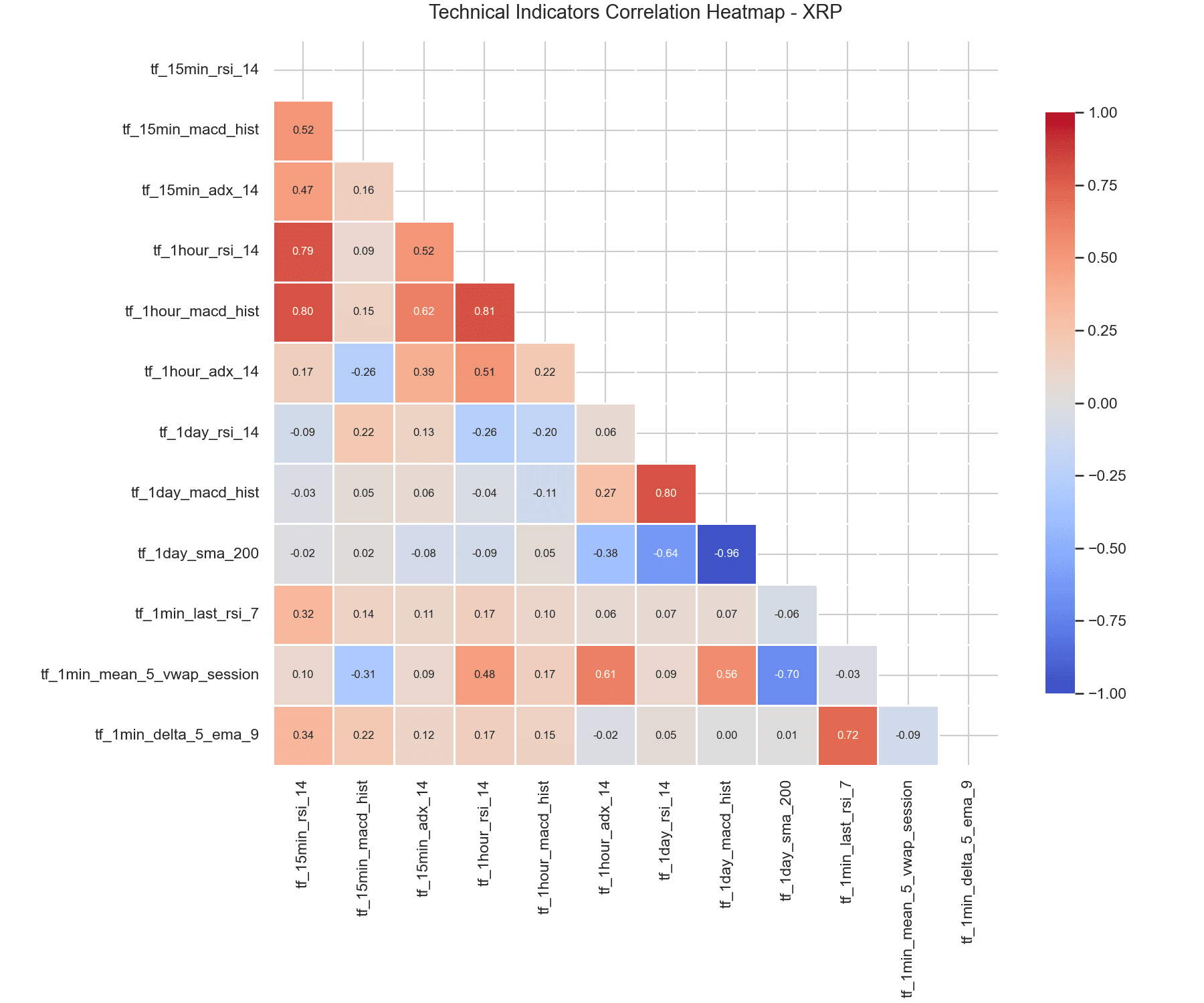 |
Indicators of similar frequencies show moderate correlation (e.g. r ≈ 0.65 between 15-minute and 1-hour RSI), but short-term 1-minute indicators are decoupled from hourly and daily trends. This structure lets the models combine microstructural mean-reversion signals with medium-term directional momentum without suffering from multicollinearity.
7. Computational Hardware Environment
To ensure complete transparency, all experiments were executed on a local workstation containing an Intel(R) Core(TM) Ultra 9 275HX CPU (24 Cores) and an NVIDIA GeForce RTX 5080 Laptop GPU.
8. Conclusion
This study demonstrates that Google Research’s TabFM zero-shot tabular foundation model is capable of predicting short-horizon prediction markets. By leveraging pre-trained representations and in-context learning with a 120-row historical window, TabFM achieved a competitive 53.86% accuracy on XRP, outperforming the fully trained XGBoost baseline on that asset.
Logistic Regression coefficients and SHAP values show that Polymarket outcomes on these 5-minute crypto contracts are driven by a combination of trend momentum (RSI), trend exhaustion (MACD), and mean reversion (session VWAP). Tabular foundation models carry higher computational latency from the transformer’s forward pass, but their zero-shot capability — skipping training entirely — is a genuinely useful alternative to standing up a full model-training pipeline for short-horizon financial forecasting.
None of the accuracies above clear a large enough margin over a 50% coin flip to be treated as a standalone edge before transaction costs, market impact, and Polymarket’s fee structure are accounted for. This is a research screen into what drives these markets, not a validated trading signal.
9. Replication Code
Replication code is provided below in collapsible dropdowns.
Click to view run_tabfm_prediction.py (TabFM Backtest Script)
"""
Walk-forward TabFM evaluation for Polymarket modeling datasets.

Outputs:
  polymarket_blogposts/results/<RUN_LABEL>/<SYMBOL>/historical_predictions.parquet
  polymarket_blogposts/results/<RUN_LABEL>/<SYMBOL>/confusion_matrix.csv
  polymarket_blogposts/results/<RUN_LABEL>/<SYMBOL>/summary.json
  polymarket_blogposts/results/<RUN_LABEL>/run_summary.json
"""

from __future__ import annotations

import argparse
import json
import logging
import math
import sys
import time
from pathlib import Path
from typing import Any

import pandas as pd
import numpy as np
from sklearn.metrics import accuracy_score, confusion_matrix, f1_score, precision_score, recall_score, roc_auc_score

# Ensure the local tabfm package is on path
BLOGPOSTS_DIR = Path(__file__).resolve().parent
sys.path.insert(0, str(BLOGPOSTS_DIR / "tabfm"))

from tabfm import TabFMClassifier
from tabfm.src.pytorch import tabfm_v1_0_0 as tabfm_v1_0_0_pytorch

# Paths to datasets
TRADING_PROJECT_DIR = Path("C:/Users/MattO/Documents/projects_V2/2026/trading_polymarket_crypto_prediction")
DATA_ROOT = TRADING_PROJECT_DIR / "xgboost" / "data"
OUTPUT_ROOT = BLOGPOSTS_DIR / "results"
SYMBOLS = ["BTC", "ETH", "XRP"]

logging.basicConfig(
    level=logging.INFO,
    format="%(asctime)s  %(levelname)-8s  %(message)s",
    datefmt="%Y-%m-%d %H:%M:%S",
    handlers=[logging.StreamHandler(sys.stdout)],
)
log = logging.getLogger(__name__)


def _write_json(path: Path, payload: dict[str, Any]) -> None:
    path.parent.mkdir(parents=True, exist_ok=True)
    with open(path, "w", encoding="utf-8") as handle:
        json.dump(payload, handle, indent=2, ensure_ascii=True)
        handle.write("\n")


def _parse_symbols(raw: str) -> list[str]:
    requested = [part.strip().upper() for part in raw.split(",") if part.strip()]
    invalid = [symbol for symbol in requested if symbol not in SYMBOLS]
    if invalid:
        raise ValueError(f"Unsupported symbols: {', '.join(invalid)}")
    return requested or SYMBOLS


def _load_dataset(symbol: str) -> pd.DataFrame:
    path = DATA_ROOT / symbol / "combined" / "modeling.parquet"
    if not path.exists():
        raise FileNotFoundError(f"Missing modeling dataset: {path}")

    df = pd.read_parquet(path)
    if df.empty:
        return df

    df["time"] = pd.to_datetime(df["time"], errors="coerce", utc=True)
    df["target_up_binary"] = pd.to_numeric(df["target_up_binary"], errors="coerce")
    df = df.dropna(subset=["time", "target_up_binary"]).sort_values("time").drop_duplicates(subset=["time"], keep="last").reset_index(drop=True)

    # Fill any missing indicator values before feeding to TabFM
    df = df.ffill().bfill()
    return df


def _select_features(df: pd.DataFrame, mode: str) -> list[str]:
    all_features = [col for col in df.columns if col not in ["time", "target_up_binary"]]

    if mode == "all":
        return all_features
    elif mode == "key":
        # Curate 12 key indicators representing different periods and categories
        key_patterns = [
            "tf_15min_rsi_14",
            "tf_15min_macd_hist",
            "tf_15min_adx_14",
            "tf_1hour_rsi_14",
            "tf_1hour_macd_hist",
            "tf_1hour_adx_14",
            "tf_1day_rsi_14",
            "tf_1day_macd_hist",
            "tf_1day_sma_200",
            "tf_1min_last_rsi_7",
            "tf_1min_mean_5_vwap_session",
            "tf_1min_delta_5_ema_9"
        ]
        selected = [col for col in key_patterns if col in df.columns]
        if not selected:
            log.warning("No key features matched, falling back to first 10 columns.")
            return all_features[:10]
        return selected
    else:
        raise ValueError(f"Unknown feature mode: {mode}")


def _build_folds(n_rows: int, min_train_size: int, test_size: int, step_size: int, min_last_test_size: int) -> list[tuple[int, int, int]]:
    folds: list[tuple[int, int, int]] = []
    fold_id = 1
    train_end = min_train_size

    while train_end < n_rows:
        test_end = min(train_end + test_size, n_rows)
        if test_end - train_end < min_last_test_size:
            break
        folds.append((fold_id, train_end, test_end))
        fold_id += 1
        train_end += step_size

    return folds


def _fit_and_predict(
    X_train: pd.DataFrame,
    y_train: pd.Series,
    X_test: pd.DataFrame,
    model: Any,
    n_estimators: int,
    max_num_rows: int | None,
) -> tuple[pd.Series, pd.Series, str]:
    if y_train.nunique(dropna=True) < 2:
        constant_class = int(y_train.iloc[0])
        prob = pd.Series([float(constant_class)] * len(X_test), index=X_test.index, dtype=float)
        pred = pd.Series([constant_class] * len(X_test), index=X_test.index, dtype=int)
        return pred, prob, "constant_baseline"

    # Initialize TabFMClassifier
    clf = TabFMClassifier(
        model=model,
        n_estimators=n_estimators,
        max_num_rows=max_num_rows,
        random_state=42,
        verbose=False,
    )
    clf.fit(X_train.to_numpy(), y_train.to_numpy())

    probs = clf.predict_proba(X_test.to_numpy())
    prob = pd.Series(probs[:, 1], index=X_test.index, dtype=float)
    pred = pd.Series(clf.predict(X_test.to_numpy()), index=X_test.index, dtype=int)
    return pred, prob, "tabfm"


def _metrics_payload(y_true: pd.Series, y_pred: pd.Series, y_prob: pd.Series) -> dict[str, Any]:
    payload: dict[str, Any] = {
        "rows": int(len(y_true)),
        "accuracy": float(accuracy_score(y_true, y_pred)),
        "precision_up": float(precision_score(y_true, y_pred, zero_division=0)),
        "recall_up": float(recall_score(y_true, y_pred, zero_division=0)),
        "f1_up": float(f1_score(y_true, y_pred, zero_division=0)),
    }
    try:
        payload["roc_auc"] = float(roc_auc_score(y_true, y_prob))
    except ValueError:
        payload["roc_auc"] = None
    return payload


def _confusion_frame(y_true: pd.Series, y_pred: pd.Series) -> pd.DataFrame:
    matrix = confusion_matrix(y_true, y_pred, labels=[0, 1])
    return pd.DataFrame(
        matrix,
        index=["actual_down_0", "actual_up_1"],
        columns=["pred_down_0", "pred_up_1"],
    )


def _evaluate_symbol(
    symbol: str,
    model: Any,
    run_dir: Path,
    min_train_size: int,
    test_size: int,
    step_size: int,
    min_last_test_size: int,
    feature_mode: str,
    n_estimators: int,
    max_num_rows: int | None,
    fast_test: bool,
) -> tuple[pd.DataFrame, dict[str, Any]]:
    df = _load_dataset(symbol)
    feature_columns = _select_features(df, feature_mode)
    feature_df = df[feature_columns].copy()
    target = df["target_up_binary"].astype(int)

    folds = _build_folds(
        n_rows=len(df),
        min_train_size=min_train_size,
        test_size=test_size,
        step_size=step_size,
        min_last_test_size=min_last_test_size,
    )
    if not folds:
        raise RuntimeError(f"Not enough rows to create walk-forward folds for {symbol}")

    if fast_test:
        log.info("Fast test mode enabled: running only the first 2 folds")
        folds = folds[:2]

    prediction_parts: list[pd.DataFrame] = []
    fold_rows: list[dict[str, Any]] = []

    for fold_idx, (fold_id, train_end, test_end) in enumerate(folds):
        t0 = time.time()

        train_index = feature_df.index[:train_end]
        test_index = feature_df.index[train_end:test_end]

        X_train = feature_df.loc[train_index]
        y_train = target.loc[train_index]
        X_test = feature_df.loc[test_index]
        y_test = target.loc[test_index]

        y_pred, y_prob, model_type = _fit_and_predict(
            X_train, y_train, X_test, model, n_estimators=n_estimators, max_num_rows=max_num_rows
        )

        dt = time.time() - t0
        log.info(
            "Symbol=%s Fold=%d/%d (%d train rows, %d test rows) completed in %.2fs",
            symbol,
            fold_id,
            len(folds),
            len(train_index),
            len(test_index),
            dt,
        )

        part = pd.DataFrame(
            {
                "time": df.loc[test_index, "time"].values,
                "symbol": symbol,
                "fold_id": fold_id,
                "model_type": model_type,
                "y_true": y_test.values,
                "y_pred": y_pred.values,
                "y_prob_up": y_prob.values,
                "train_rows": len(train_index),
                "test_rows": len(test_index),
            }
        )
        prediction_parts.append(part)

        fold_metrics = _metrics_payload(y_test, y_pred, y_prob)
        fold_metrics.update(
            {
                "fold_id": fold_id,
                "model_type": model_type,
                "train_rows": len(train_index),
                "test_rows": len(test_index),
            }
        )
        fold_rows.append(fold_metrics)

    predictions = pd.concat(prediction_parts, ignore_index=True).sort_values("time").reset_index(drop=True)
    predictions["correct"] = (predictions["y_true"] == predictions["y_pred"]).astype(int)

    fold_metrics_df = pd.DataFrame(fold_rows)
    confusion_df = _confusion_frame(predictions["y_true"], predictions["y_pred"])

    summary = {
        "symbol": symbol,
        "dataset_rows": int(len(df)),
        "feature_columns": int(len(feature_columns)),
        "predicted_rows": int(len(predictions)),
        "folds": int(len(folds)),
        "min_train_size": min_train_size,
        "test_size": test_size,
        "step_size": step_size,
        "n_estimators": n_estimators,
        "max_num_rows": max_num_rows,
        "feature_mode": feature_mode,
    }
    summary.update(_metrics_payload(predictions["y_true"], predictions["y_pred"], predictions["y_prob_up"]))

    symbol_dir = run_dir / symbol
    symbol_dir.mkdir(parents=True, exist_ok=True)
    predictions.to_parquet(symbol_dir / "historical_predictions.parquet", index=False)
    fold_metrics_df.to_csv(symbol_dir / "fold_metrics.csv", index=False)
    confusion_df.to_csv(symbol_dir / "confusion_matrix.csv")
    _write_json(symbol_dir / "summary.json", summary)

    _write_json(
        symbol_dir / "confusion_matrix.json",
        {
            "actual_down_0": {
                "pred_down_0": int(confusion_df.loc["actual_down_0", "pred_down_0"]),
                "pred_up_1": int(confusion_df.loc["actual_down_0", "pred_up_1"]),
            },
            "actual_up_1": {
                "pred_down_0": int(confusion_df.loc["actual_up_1", "pred_down_0"]),
                "pred_up_1": int(confusion_df.loc["actual_up_1", "pred_up_1"]),
            },
        },
    )

    return predictions, summary


def parse_args() -> argparse.Namespace:
    parser = argparse.ArgumentParser(description="Walk-forward TabFM evaluation.")
    parser.add_argument("--symbols", default="BTC,ETH,XRP", help="Comma-separated symbols to evaluate.")
    parser.add_argument("--run-label", default="tabfm_key_features", help="Output subfolder label.")
    parser.add_argument("--min-train-size", type=int, default=120, help="Initial training rows per symbol.")
    parser.add_argument("--test-size", type=int, default=24, help="Rows per test fold.")
    parser.add_argument("--step-size", type=int, default=24, help="How far to advance the expanding window per fold.")
    parser.add_argument("--min-last-test-size", type=int, default=12, help="Minimum size for the last partial fold.")
    parser.add_argument("--feature-mode", default="key", choices=["key", "all"], help="Feature selection mode.")
    parser.add_argument("--n-estimators", type=int, default=8, help="Number of TabFM ensemble estimators.")
    parser.add_argument("--max-num-rows", type=int, default=120, help="Max in-context training rows (None for all).")
    parser.add_argument("--fast-test", action="store_true", help="Only run 2 folds for testing setup.")
    return parser.parse_args()


def main() -> None:
    args = parse_args()
    symbols = _parse_symbols(args.symbols)
    run_dir = OUTPUT_ROOT / args.run_label
    run_dir.mkdir(parents=True, exist_ok=True)

    log.info("Loading PyTorch TabFM model...")
    t_start_load = time.time()
    model = tabfm_v1_0_0_pytorch.load(model_type='classification', device='cpu')
    log.info("TabFM model loaded in %.2fs", time.time() - t_start_load)

    combined_predictions: list[pd.DataFrame] = []
    run_summary: dict[str, Any] = {
        "run_label": args.run_label,
        "symbols": {},
        "timestamp": time.strftime("%Y-%m-%d %H:%M:%S")
    }

    for symbol in symbols:
        log.info("Evaluating symbol %s...", symbol)
        predictions, summary = _evaluate_symbol(
            symbol=symbol,
            model=model,
            run_dir=run_dir,
            min_train_size=args.min_train_size,
            test_size=args.test_size,
            step_size=args.step_size,
            min_last_test_size=args.min_last_test_size,
            feature_mode=args.feature_mode,
            n_estimators=args.n_estimators,
            max_num_rows=args.max_num_rows,
            fast_test=args.fast_test,
        )
        combined_predictions.append(predictions)
        run_summary["symbols"][symbol] = summary
        log.info(
            "%s walk-forward complete: predicted_rows=%d accuracy=%.4f",
            symbol,
            summary["predicted_rows"],
            summary["accuracy"],
        )

    combined_df = pd.concat(combined_predictions, ignore_index=True).sort_values(["symbol", "time"]).reset_index(drop=True)
    combined_df.to_parquet(run_dir / "combined_historical_predictions.parquet", index=False)

    combined_confusion = _confusion_frame(combined_df["y_true"], combined_df["y_pred"])
    combined_confusion.to_csv(run_dir / "combined_confusion_matrix.csv")

    overall = {
        "run_label": args.run_label,
        "symbols": symbols,
        "predicted_rows": int(len(combined_df)),
    }
    overall.update(_metrics_payload(combined_df["y_true"], combined_df["y_pred"], combined_df["y_prob_up"]))
    run_summary["overall"] = overall
    _write_json(run_dir / "run_summary.json", run_summary)

    log.info("Combined walk-forward summary written to %s", run_dir)
    log.info("Overall Accuracy: %.4f | Precision (Up): %.4f | Recall (Up): %.4f",
             overall["accuracy"], overall["precision_up"], overall["recall_up"])


if __name__ == "__main__":
    main()
Click to view run_baseline_models.py (Traditional Baselines Script)
"""
Walk-forward evaluation of standard baseline models:
- Logistic Regression
- Random Forest
- Support Vector Machine (SVM)

Outputs:
  polymarket_blogposts/results/baselines/<SYMBOL>/historical_predictions_<MODEL>.parquet
  polymarket_blogposts/results/baselines/<SYMBOL>/summary_<MODEL>.json
  polymarket_blogposts/results/baselines/<SYMBOL>/feature_importances_rf.csv
  polymarket_blogposts/results/baselines/<SYMBOL>/coefficients_lr.csv
  polymarket_blogposts/results/baselines/run_summary.json
"""

import argparse
import json
import logging
import math
import sys
import time
from pathlib import Path
from typing import Any

import pandas as pd
import numpy as np
from sklearn.linear_model import LogisticRegression
from sklearn.ensemble import RandomForestClassifier
from sklearn.svm import SVC
from sklearn.preprocessing import StandardScaler
from sklearn.metrics import accuracy_score, confusion_matrix, f1_score, precision_score, recall_score, roc_auc_score

# Paths to datasets
TRADING_PROJECT_DIR = Path("C:/Users/MattO/Documents/projects_V2/2026/trading_polymarket_crypto_prediction")
DATA_ROOT = TRADING_PROJECT_DIR / "xgboost" / "data"
OUTPUT_ROOT = Path(__file__).resolve().parent / "results" / "baselines"
SYMBOLS = ["BTC", "ETH", "XRP"]

logging.basicConfig(
    level=logging.INFO,
    format="%(asctime)s  %(levelname)-8s  %(message)s",
    datefmt="%Y-%m-%d %H:%M:%S",
    handlers=[logging.StreamHandler(sys.stdout)],
)
log = logging.getLogger(__name__)


def _write_json(path: Path, payload: dict[str, Any]) -> None:
    path.parent.mkdir(parents=True, exist_ok=True)
    with open(path, "w", encoding="utf-8") as handle:
        json.dump(payload, handle, indent=2, ensure_ascii=True)
        handle.write("\n")


def _parse_symbols(raw: str) -> list[str]:
    requested = [part.strip().upper() for part in raw.split(",") if part.strip()]
    invalid = [symbol for symbol in requested if symbol not in SYMBOLS]
    if invalid:
        raise ValueError(f"Unsupported symbols: {', '.join(invalid)}")
    return requested or SYMBOLS


def _load_dataset(symbol: str) -> pd.DataFrame:
    path = DATA_ROOT / symbol / "combined" / "modeling.parquet"
    if not path.exists():
        raise FileNotFoundError(f"Missing modeling dataset: {path}")

    df = pd.read_parquet(path)
    if df.empty:
        return df

    df["time"] = pd.to_datetime(df["time"], errors="coerce", utc=True)
    df["target_up_binary"] = pd.to_numeric(df["target_up_binary"], errors="coerce")
    df = df.dropna(subset=["time", "target_up_binary"]).sort_values("time").drop_duplicates(subset=["time"], keep="last").reset_index(drop=True)

    # Fill any missing indicator values
    df = df.ffill().bfill()
    return df


def _select_features(df: pd.DataFrame, mode: str) -> list[str]:
    all_features = [col for col in df.columns if col not in ["time", "target_up_binary"]]

    if mode == "all":
        return all_features
    elif mode == "key":
        key_patterns = [
            "tf_15min_rsi_14",
            "tf_15min_macd_hist",
            "tf_15min_adx_14",
            "tf_1hour_rsi_14",
            "tf_1hour_macd_hist",
            "tf_1hour_adx_14",
            "tf_1day_rsi_14",
            "tf_1day_macd_hist",
            "tf_1day_sma_200",
            "tf_1min_last_rsi_7",
            "tf_1min_mean_5_vwap_session",
            "tf_1min_delta_5_ema_9"
        ]
        selected = [col for col in key_patterns if col in df.columns]
        if not selected:
            return all_features[:10]
        return selected
    else:
        raise ValueError(f"Unknown feature mode: {mode}")


def _build_folds(n_rows: int, min_train_size: int, test_size: int, step_size: int, min_last_test_size: int) -> list[tuple[int, int, int]]:
    folds: list[tuple[int, int, int]] = []
    fold_id = 1
    train_end = min_train_size

    while train_end < n_rows:
        test_end = min(train_end + test_size, n_rows)
        if test_end - train_end < min_last_test_size:
            break
        folds.append((fold_id, train_end, test_end))
        fold_id += 1
        train_end += step_size

    return folds


def _metrics_payload(y_true: pd.Series, y_pred: pd.Series, y_prob: pd.Series) -> dict[str, Any]:
    payload: dict[str, Any] = {
        "rows": int(len(y_true)),
        "accuracy": float(accuracy_score(y_true, y_pred)),
        "precision_up": float(precision_score(y_true, y_pred, zero_division=0)),
        "recall_up": float(recall_score(y_true, y_pred, zero_division=0)),
        "f1_up": float(f1_score(y_true, y_pred, zero_division=0)),
    }
    try:
        payload["roc_auc"] = float(roc_auc_score(y_true, y_prob))
    except ValueError:
        payload["roc_auc"] = None
    return payload


def _confusion_frame(y_true: pd.Series, y_pred: pd.Series) -> pd.DataFrame:
    matrix = confusion_matrix(y_true, y_pred, labels=[0, 1])
    return pd.DataFrame(
        matrix,
        index=["actual_down_0", "actual_up_1"],
        columns=["pred_down_0", "pred_up_1"],
    )


def _get_model(name: str) -> Any:
    if name == "lr":
        return LogisticRegression(C=0.1, max_iter=1000, random_state=42)
    elif name == "rf":
        return RandomForestClassifier(n_estimators=100, max_depth=5, min_samples_leaf=2, random_state=42)
    elif name == "svm":
        return SVC(C=1.0, kernel="rbf", probability=True, random_state=42)
    else:
        raise ValueError(f"Unknown model name: {name}")


def _evaluate_model_symbol(
    symbol: str,
    model_name: str,
    df: pd.DataFrame,
    feature_df: pd.DataFrame,
    target: pd.Series,
    folds: list[tuple[int, int, int]],
    symbol_dir: Path,
) -> tuple[pd.DataFrame, dict[str, Any]]:
    prediction_parts = []

    for fold_id, train_end, test_end in folds:
        train_index = feature_df.index[:train_end]
        test_index = feature_df.index[train_end:test_end]

        X_train = feature_df.loc[train_index]
        y_train = target.loc[train_index]
        X_test = feature_df.loc[test_index]
        y_test = target.loc[test_index]

        # Standardize for models that need it (LR, SVM)
        scaler = StandardScaler()
        X_train_scaled = scaler.fit_transform(X_train)
        X_test_scaled = scaler.transform(X_test)

        model = _get_model(model_name)

        # Fit models
        if model_name in ["lr", "svm"]:
            model.fit(X_train_scaled, y_train)
            probs = model.predict_proba(X_test_scaled)[:, 1]
            preds = model.predict(X_test_scaled)
        else:
            model.fit(X_train, y_train)
            probs = model.predict_proba(X_test)[:, 1]
            preds = model.predict(X_test)

        part = pd.DataFrame(
            {
                "time": df.loc[test_index, "time"].values,
                "symbol": symbol,
                "fold_id": fold_id,
                "y_true": y_test.values,
                "y_pred": preds,
                "y_prob_up": probs,
            }
        )
        prediction_parts.append(part)

    predictions = pd.concat(prediction_parts, ignore_index=True).sort_values("time").reset_index(drop=True)
    metrics = _metrics_payload(predictions["y_true"], predictions["y_pred"], predictions["y_prob_up"])

    # Save predictions & metrics
    predictions.to_parquet(symbol_dir / f"historical_predictions_{model_name}.parquet", index=False)

    summary = {
        "symbol": symbol,
        "model": model_name,
        "predicted_rows": int(len(predictions)),
        **metrics
    }
    _write_json(symbol_dir / f"summary_{model_name}.json", summary)

    return predictions, summary


def _analyze_importances(
    symbol: str,
    feature_df: pd.DataFrame,
    target: pd.Series,
    symbol_dir: Path,
) -> None:
    """Train models on full dataset to analyze feature importances / coefficients."""
    log.info("Analyzing feature importances on full dataset for %s...", symbol)

    # Scale data for Logistic Regression
    scaler = StandardScaler()
    feature_scaled = scaler.fit_transform(feature_df)

    # Logistic Regression Analysis
    lr = LogisticRegression(C=0.1, max_iter=1000, random_state=42)
    lr.fit(feature_scaled, target)

    coef_df = pd.DataFrame({
        "feature": feature_df.columns,
        "coefficient": lr.coef_[0],
        "abs_coefficient": np.abs(lr.coef_[0])
    }).sort_values("abs_coefficient", ascending=False).reset_index(drop=True)

    coef_df.to_csv(symbol_dir / "coefficients_lr.csv", index=False)
    log.info("Logistic Regression top variables for %s:\n%s", symbol, coef_df.head(5).to_string())

    # Random Forest Analysis
    rf = RandomForestClassifier(n_estimators=100, max_depth=5, min_samples_leaf=2, random_state=42)
    rf.fit(feature_df, target)

    rf_df = pd.DataFrame({
        "feature": feature_df.columns,
        "importance": rf.feature_importances_
    }).sort_values("importance", ascending=False).reset_index(drop=True)

    rf_df.to_csv(symbol_dir / "feature_importances_rf.csv", index=False)
    log.info("Random Forest top variables for %s:\n%s", symbol, rf_df.head(5).to_string())


def main() -> None:
    parser = argparse.ArgumentParser(description="Evaluate baseline models (LR, RF, SVM).")
    parser.add_argument("--symbols", default="BTC,ETH,XRP", help="Comma-separated symbols.")
    parser.add_argument("--min-train-size", type=int, default=120, help="Initial training size.")
    parser.add_argument("--test-size", type=int, default=24, help="Test fold size.")
    parser.add_argument("--step-size", type=int, default=24, help="Step size.")
    parser.add_argument("--min-last-test-size", type=int, default=12, help="Min last fold size.")
    parser.add_argument("--feature-mode", default="key", choices=["key", "all"], help="Feature selection mode.")
    args = parser.parse_args()

    symbols = _parse_symbols(args.symbols)
    OUTPUT_ROOT.mkdir(parents=True, exist_ok=True)

    run_summary: dict[str, Any] = {
        "timestamp": time.strftime("%Y-%m-%d %H:%M:%S"),
        "symbols": {}
    }

    for symbol in symbols:
        log.info("Starting baseline evaluations for %s...", symbol)
        df = _load_dataset(symbol)
        feature_columns = _select_features(df, args.feature_mode)
        feature_df = df[feature_columns].copy()
        target = df["target_up_binary"].astype(int)

        folds = _build_folds(
            n_rows=len(df),
            min_train_size=args.min_train_size,
            test_size=args.test_size,
            step_size=args.step_size,
            min_last_test_size=args.min_last_test_size,
        )

        symbol_dir = OUTPUT_ROOT / symbol
        symbol_dir.mkdir(parents=True, exist_ok=True)

        run_summary["symbols"][symbol] = {}

        # Run evaluations
        for model_name in ["lr", "rf", "svm"]:
            log.info("Running walk-forward for %s model on %s...", model_name.upper(), symbol)
            _, summary = _evaluate_model_symbol(
                symbol=symbol,
                model_name=model_name,
                df=df,
                feature_df=feature_df,
                target=target,
                folds=folds,
                symbol_dir=symbol_dir,
            )
            run_summary["symbols"][symbol][model_name] = summary
            log.info(
                "%s model on %s complete: Accuracy = %.4f",
                model_name.upper(), symbol, summary["accuracy"]
            )

        # Run feature importance analysis
        _analyze_importances(symbol, feature_df, target, symbol_dir)

    _write_json(OUTPUT_ROOT / "run_summary.json", run_summary)
    log.info("Baseline evaluations complete. Outputs saved in %s", OUTPUT_ROOT)


if __name__ == "__main__":
    main()
Click to view generate_analysis.py (Plotting & Analysis Script)
"""
Generate feature analysis visualizations:
- Logistic Regression Coefficients Bar Plot
- Random Forest Feature Importances Bar Plot
- SHAP Summary (Beeswarm) Plot
- Correlation Heatmap

Outputs:
  polymarket_blogposts/results/analysis/<SYMBOL>/coefficients_lr.png
  polymarket_blogposts/results/analysis/<SYMBOL>/feature_importances_rf.png
  polymarket_blogposts/results/analysis/<SYMBOL>/shap_summary_rf.png
  polymarket_blogposts/results/analysis/<SYMBOL>/feature_correlation.png
"""

import logging
import sys
from pathlib import Path

import pandas as pd
import numpy as np
import matplotlib.pyplot as plt
import seaborn as sns
from sklearn.linear_model import LogisticRegression
from sklearn.ensemble import RandomForestClassifier
from sklearn.preprocessing import StandardScaler
import shap

# Ensure clean plotting on headless systems
matplotlib_logger = logging.getLogger("matplotlib")
matplotlib_logger.setLevel(logging.WARNING)

# Paths to datasets
TRADING_PROJECT_DIR = Path("C:/Users/MattO/Documents/projects_V2/2026/trading_polymarket_crypto_prediction")
DATA_ROOT = TRADING_PROJECT_DIR / "xgboost" / "data"
OUTPUT_ROOT = Path(__file__).resolve().parent / "results" / "analysis"
SYMBOLS = ["BTC", "ETH", "XRP"]

logging.basicConfig(
    level=logging.INFO,
    format="%(asctime)s  %(levelname)-8s  %(message)s",
    datefmt="%Y-%m-%d %H:%M:%S",
    handlers=[logging.StreamHandler(sys.stdout)],
)
log = logging.getLogger(__name__)


def _load_dataset(symbol: str) -> pd.DataFrame:
    path = DATA_ROOT / symbol / "combined" / "modeling.parquet"
    if not path.exists():
        raise FileNotFoundError(f"Missing modeling dataset: {path}")

    df = pd.read_parquet(path)
    if df.empty:
        return df

    df["time"] = pd.to_datetime(df["time"], errors="coerce", utc=True)
    df["target_up_binary"] = pd.to_numeric(df["target_up_binary"], errors="coerce")
    df = df.dropna(subset=["time", "target_up_binary"]).sort_values("time").drop_duplicates(subset=["time"], keep="last").reset_index(drop=True)
    df = df.ffill().bfill()
    return df


def _select_features(df: pd.DataFrame) -> list[str]:
    key_patterns = [
        "tf_15min_rsi_14",
        "tf_15min_macd_hist",
        "tf_15min_adx_14",
        "tf_1hour_rsi_14",
        "tf_1hour_macd_hist",
        "tf_1hour_adx_14",
        "tf_1day_rsi_14",
        "tf_1day_macd_hist",
        "tf_1day_sma_200",
        "tf_1min_last_rsi_7",
        "tf_1min_mean_5_vwap_session",
        "tf_1min_delta_5_ema_9"
    ]
    selected = [col for col in key_patterns if col in df.columns]
    if not selected:
        all_features = [col for col in df.columns if col not in ["time", "target_up_binary"]]
        return all_features[:12]
    return selected


def _plot_lr_coefficients(coef_df: pd.DataFrame, out_path: Path, symbol: str) -> None:
    plt.figure(figsize=(10, 6))
    # Sort by coefficient value
    sorted_df = coef_df.sort_values("coefficient", ascending=True)

    # Custom color palette: red for negative, green for positive
    colors = ["#e74c3c" if c < 0 else "#2ecc71" for c in sorted_df["coefficient"]]

    sns.barplot(
        x="coefficient",
        y="feature",
        data=sorted_df,
        palette=colors,
        hue="feature",
        legend=False
    )
    plt.axvline(x=0, color="#2c3e50", linestyle="--", linewidth=1)
    plt.title(f"Logistic Regression Coefficients - {symbol}\n(Predicting Market Resolving UP)", fontsize=14, pad=15)
    plt.xlabel("Coefficient Value (Feature Weight)", fontsize=12)
    plt.ylabel("Technical Indicator Feature", fontsize=12)
    plt.grid(axis="x", linestyle=":", alpha=0.6)
    plt.tight_layout()
    plt.savefig(out_path, dpi=150)
    plt.close()


def _plot_rf_importances(importance_df: pd.DataFrame, out_path: Path, symbol: str) -> None:
    plt.figure(figsize=(10, 6))
    sorted_df = importance_df.sort_values("importance", ascending=True)

    sns.barplot(
        x="importance",
        y="feature",
        data=sorted_df,
        palette="viridis",
        hue="feature",
        legend=False
    )
    plt.title(f"Random Forest Gini Feature Importances - {symbol}", fontsize=14, pad=15)
    plt.xlabel("Gini Importance Score", fontsize=12)
    plt.ylabel("Technical Indicator Feature", fontsize=12)
    plt.grid(axis="x", linestyle=":", alpha=0.6)
    plt.tight_layout()
    plt.savefig(out_path, dpi=150)
    plt.close()


def _plot_shap_summary(rf: RandomForestClassifier, X: pd.DataFrame, out_path: Path, symbol: str) -> None:
    try:
        explainer = shap.TreeExplainer(rf)
        shap_values = explainer.shap_values(X)

        # Determine correct indexing for binary classification SHAP values
        if isinstance(shap_values, list):
            # Old SHAP format (list of two arrays, one per class)
            # Use class 1 (UP)
            shap_vals_to_use = shap_values[1]
        elif isinstance(shap_values, np.ndarray) and len(shap_values.shape) == 3:
            # Shape is (samples, features, classes)
            shap_vals_to_use = shap_values[:, :, 1]
        else:
            shap_vals_to_use = shap_values

        plt.figure(figsize=(10, 6))
        # shap.summary_plot generates its own figure elements
        shap.summary_plot(shap_vals_to_use, X, show=False)
        plt.title(f"SHAP Summary (Random Forest UP Class) - {symbol}", fontsize=14, pad=15)
        plt.tight_layout()
        plt.savefig(out_path, dpi=150)
        plt.close()
    except Exception as e:
        log.error("Failed to generate SHAP summary for %s: %s", symbol, e)


def _plot_correlation_matrix(feature_df: pd.DataFrame, out_path: Path, symbol: str) -> None:
    plt.figure(figsize=(12, 10))
    corr = feature_df.corr()

    # Generate a mask for the upper triangle
    mask = np.triu(np.ones_like(corr, dtype=bool))

    sns.heatmap(
        corr,
        mask=mask,
        cmap="coolwarm",
        vmax=1.0,
        vmin=-1.0,
        center=0,
        square=True,
        linewidths=0.5,
        cbar_kws={"shrink": 0.8},
        annot=True,
        fmt=".2f",
        annot_kws={"size": 8}
    )
    plt.title(f"Technical Indicators Correlation Heatmap - {symbol}", fontsize=14, pad=15)
    plt.tight_layout()
    plt.savefig(out_path, dpi=150)
    plt.close()


def main() -> None:
    OUTPUT_ROOT.mkdir(parents=True, exist_ok=True)
    sns.set_theme(style="whitegrid")

    for symbol in SYMBOLS:
        log.info("Processing visualization analysis for %s...", symbol)
        df = _load_dataset(symbol)
        feature_columns = _select_features(df)
        feature_df = df[feature_columns].copy()
        target = df["target_up_binary"].astype(int)

        symbol_dir = OUTPUT_ROOT / symbol
        symbol_dir.mkdir(parents=True, exist_ok=True)

        # Scale data for Logistic Regression
        scaler = StandardScaler()
        X_scaled = scaler.fit_transform(feature_df)

        # 1. Fit Logistic Regression
        lr = LogisticRegression(C=0.1, max_iter=1000, random_state=42)
        lr.fit(X_scaled, target)

        coef_df = pd.DataFrame({
            "feature": feature_df.columns,
            "coefficient": lr.coef_[0]
        })
        _plot_lr_coefficients(coef_df, symbol_dir / "coefficients_lr.png", symbol)

        # 2. Fit Random Forest
        rf = RandomForestClassifier(n_estimators=100, max_depth=5, min_samples_leaf=2, random_state=42)
        rf.fit(feature_df, target)

        importance_df = pd.DataFrame({
            "feature": feature_df.columns,
            "importance": rf.feature_importances_
        })
        _plot_rf_importances(importance_df, symbol_dir / "feature_importances_rf.png", symbol)

        # 3. Plot SHAP Summary
        _plot_shap_summary(rf, feature_df, symbol_dir / "shap_summary_rf.png", symbol)

        # 4. Plot Correlation Matrix
        _plot_correlation_matrix(feature_df, symbol_dir / "feature_correlation.png", symbol)

        log.info("Visualizations for %s generated successfully!", symbol)


if __name__ == "__main__":
    main()
Limitations
This is a research screen based on a 2-week sample window and a single historical run, not a validated trading strategy. Accuracies in the low-to-mid 50s are directionally interesting but have not been tested against Polymarket’s fee structure, execution slippage, or a longer out-of-sample period. Nothing in this article is investment advice.
Leave a Comment