Executive Summary
- Return profile: XLF earned 19.46% annualized with 15.22% volatility and a 16.61% maximum drawdown in the sample.
- Statistical edge: Weak. Variance-ratio tests do not reject a random-walk benchmark, and ARIMA selects (0,0,0), so daily return timing has not earned trust.
- Practical takeaway: Pivot from trying to predict tomorrow’s direction toward risk modeling, volatility targeting, relative strength, or explicitly backtested rules.
The conclusion is educational, not personalized financial advice. A trading strategy still needs explicit rule definitions, walk-forward validation, transaction costs, turnover, and benchmark comparisons.
Research Question
XLF is a sector-allocation question more than a pure price-pattern puzzle. Financial stocks are tied to credit, rates, liquidity, and risk appetite, so a daily standalone test can miss the real economic driver. The goal is to see whether the sample supports a basic timing rule before moving toward conditional sector exposure. This note keeps the conclusion narrow: it forms a strategy hypothesis, not a live trading recommendation.
Analysis Date And Sample Window
Table 1. Analysis Date And Sample Window
| Field | Value |
|---|---|
| Publication date | 2026-06-01 |
| Analysis run date | 2026-06-02 |
| Sample window | 2023-01-03 to 2024-12-27 |
| Return observations | 499 |
| Data fetched | 2026-06-01 |
The sample window matters. Table 1 fixes the time period before any conclusion is drawn. The analysis uses the sample ending 2024-12-27, so the statistics should be read as evidence from that window rather than a claim about today’s market state.
Return Profile
Before testing any trading rule, we need the basic risk/reward map. Table 2 shows that XLF earned 19.46% annualized with 15.22% annualized volatility and a 16.61% maximum drawdown. The zero-rate Sharpe of 1.278 compares reward with realized volatility, which helps us judge whether the sample return compensated investors for the day-to-day risk.
Table 2. Return Profile
| Metric | Value |
|---|---|
| Annualized return | 19.46% |
| Annualized volatility | 15.22% |
| Zero-rate Sharpe | 1.278 |
| Max drawdown | 16.61% |
| Lag-1 autocorrelation | 0.031 |
What this means: The return and drawdown numbers set the risk/reward backdrop for XLF. We also check lag-1 autocorrelation, which measures whether yesterday’s return carries memory into today’s return. The value of 0.031 is tiny, so yesterday’s price action gives very little help with today’s direction.
Momentum Versus Mean Reversion
The variance-ratio test in Table 3 asks whether returns behave like a random walk across different holding windows. Here, q is the return horizon in trading days, so q=4 is roughly one trading week. Quant researchers care because a value far from 1 can hint at momentum or mean reversion, but only the p-values tell us whether that hint is strong enough to trust. For XLF, VR q=2 is 1.031 with a bootstrap p-value of 0.632, q=4 is 1.117 with a p-value of 0.346, and q=16 is 1.136 with a p-value of 0.598. The heteroskedasticity-consistent statistic is unavailable in this output, so the bootstrap p-values are the inference shown here. None of the reported horizons rejects the random-walk benchmark, so the market was too efficient at these short horizons for a simple daily trend-following or mean-reversion rule to stand on its own.
Table 3. Momentum Versus Mean Reversion
| Horizon | VR | HC_Statistic | Bootstrap_p | Reject_Random_Walk |
|---|---|---|---|---|
| VR q=2 | 1.031 | n/a | 0.632 | No |
| VR q=4 | 1.117 | n/a | 0.346 | No |
| VR q=8 | 1.127 | n/a | 0.494 | No |
| VR q=16 | 1.136 | n/a | 0.598 | No |
What this means: XLF’s recent return direction did not offer a reliable clue across the tested 2, 4, 8, and 16-day windows. That is the uncomfortable reality of liquid markets: price can move strongly over a sample, yet still give very little daily timing edge. A trader can still design rules, but the rules need to prove themselves in a backtest rather than leaning on this table.
Mean-Equation Model
The mean-equation model in Table 4 asks whether daily returns have a repeatable pattern after accounting for simple time-series structure. ARIMA is useful because it tests whether past returns help explain future returns in a formal model rather than by eye. The selected ARIMA order is (0,0,0), residual Ljung-Box p-value is 0.7871, and the ARFIMA median d estimate is -0.007. For XLF, that is not a strong case for a standalone return-timing model.
Table 4. Mean-Equation Model
| Metric | Value |
|---|---|
| ARIMA order | (0,0,0) |
| ARFIMA d median | -0.007 |
| Residual Ljung-Box p | 0.7871 |
| Squared-residual Ljung-Box p | 0.0000 |
| Model conclusion | short_memory |
What this means: The mean model did not find a useful daily return equation, which means the return process offered little memory for a simple forecasting rule. The squared-residual Ljung-Box p-value of 0.0000 checks whether large moves tend to cluster after the mean model. A low value means risk has memory even if direction does not, which explains why the analysis pivots from return timing to volatility modeling.
Volatility Model Diagnostics
The volatility model in Table 5 shifts the question from direction to risk. Quants care about this because even when tomorrow’s return is hard to forecast, tomorrow’s volatility may be more predictable. That can support position sizing and stress testing, but it does not turn a weak return signal into a validated trading rule.
Table 5. Volatility Model Diagnostics
| Metric | Value |
|---|---|
| Best volatility model | gjrGARCH (sstd) |
| Persistence | 0.790 |
| Half-life | 2.942 trading days |
| Squared standardized residual p | 0.9390 |
What this means: If a volatility shock hits XLF, the fitted model estimates a half-life of about 2.9 trading days. GARCH models are built for this problem: they estimate how volatility clusters and fades after shocks. In practical terms, if a market shock doubles the asset’s volatility, a portfolio manager would expect it to take roughly this long for risk to settle halfway back toward normal, which can dictate how long to reduce position sizes.
Rolling Risk Diagnostics
The rolling-risk view in Table 6 checks whether the full-sample averages hide changing risk conditions. Quant researchers care because a strategy that looks acceptable on average can still fail if volatility, drawdown pressure, or tail behavior shifts at the wrong time.
Table 6. Rolling Risk Diagnostics
| Metric | Current | Mean | Min | Max |
|---|---|---|---|---|
| Vol 21d (ann.) | 0.147 | 0.142 | 0.069 | 0.330 |
| Vol 63d (ann.) | 0.182 | 0.143 | 0.098 | 0.232 |
| Sharpe 252d | 1.956 | 1.933 | 0.314 | 3.303 |
| Sortino 252d | 1.999 | 1.902 | 0.290 | 3.258 |
| Calmar 252d | 3.806 | 2.796 | 0.308 | 6.065 |
| ExKurtosis 60d | 8.701 | 1.002 | -0.861 | 11.895 |
What this means: Rolling risk checks whether the asset’s risk profile is stable through time. The 63-day rolling volatility is 18.16% versus a sample mean of 14.26%. The 252-day rolling Sharpe is 1.956, which shows how the risk/reward profile looked near the sample end rather than across the full window only. The 60-day excess kurtosis is 8.701, a reminder that recent large moves can cluster even when average returns look orderly. For a trader, this supports testing position sizing and volatility controls before trusting a fixed-exposure rule.
Drawdown Diagnostics
The drawdown review in Table 7 checks the realized downside path behind the strategy hypothesis. This is where a good-looking average return is forced to answer a harder question: how much pain did the investor have to sit through?
Table 7. Drawdown Diagnostics
| Metric | Value | Note | ||
|---|---|---|---|---|
| Max Drawdown | -16.27% | Trough on 2023-03-17 | ||
| Calmar Ratio | 1.196 | Strong (>1.0) | ||
| Sharpe Ratio (ann.) | 1.278 | Strong | ||
| Sortino Ratio | 1.228 | — | ||
| Ann. Volatility | 15.22% | — | ||
| #1 2023-02-08 | -16.27% | Trough 2023-03-17 | Length 27d | Recovery 186d |
| #2 2024-12-02 | -7.23% | Trough 2024-12-18 | Length 13d | Recovery Ongoingd |
| #3 2024-07-31 | -6.86% | Trough 2024-08-05 | Length 4d | Recovery 10d |
What this means: Drawdown analysis asks how much capital pain the sample required, not just how attractive the average return looked. For XLF, the maximum drawdown was 16.27%, with a Calmar ratio of 1.196 and a Sharpe ratio of 1.278. That is useful because a strategy hypothesis has to survive the bad stretches, not only the full-sample average.
Visual Evidence
The charts below come from the same statistical evidence used in the article. They are included to make the risk path easier to inspect, not to add a separate signal.
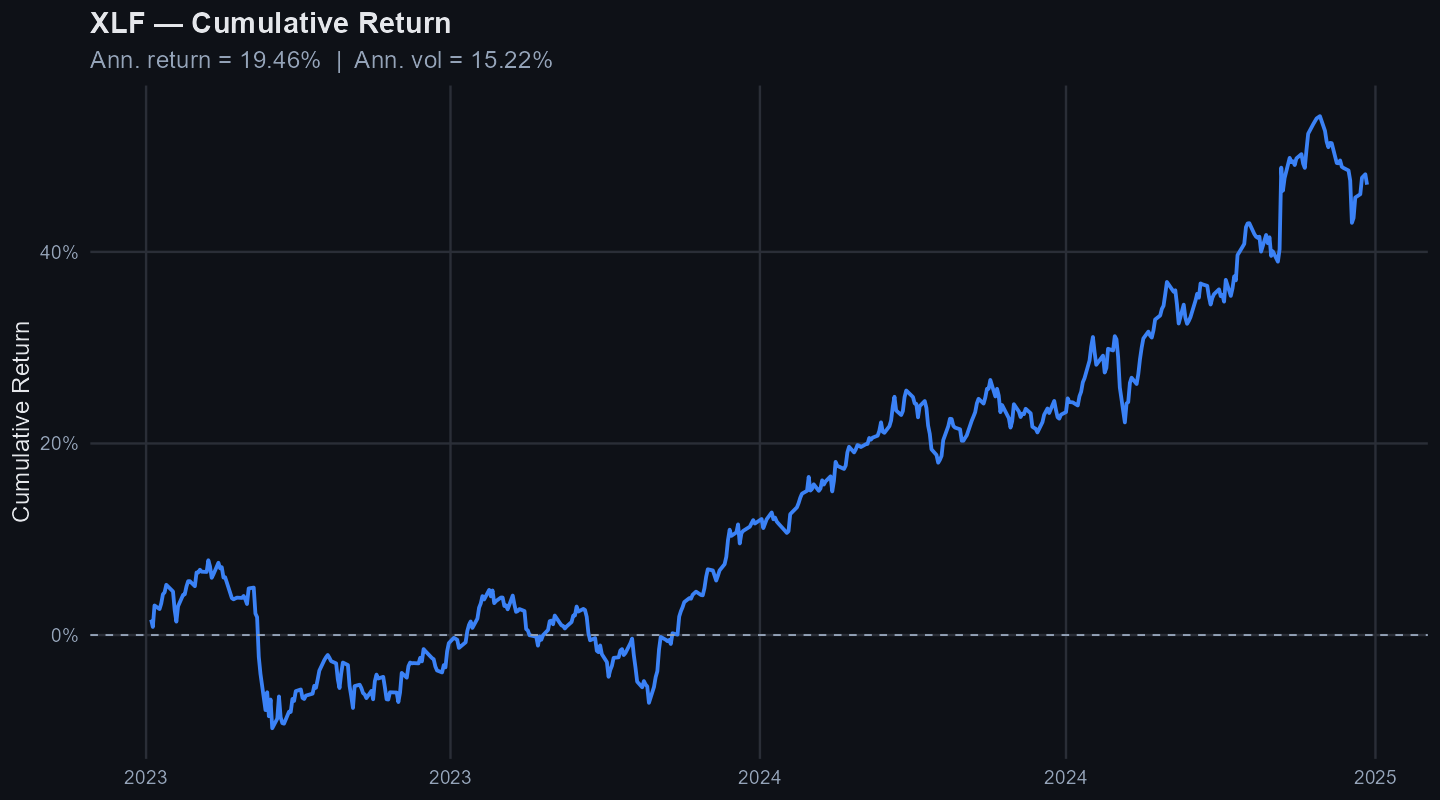
Cumulative return shows the path an investor actually had to sit through.
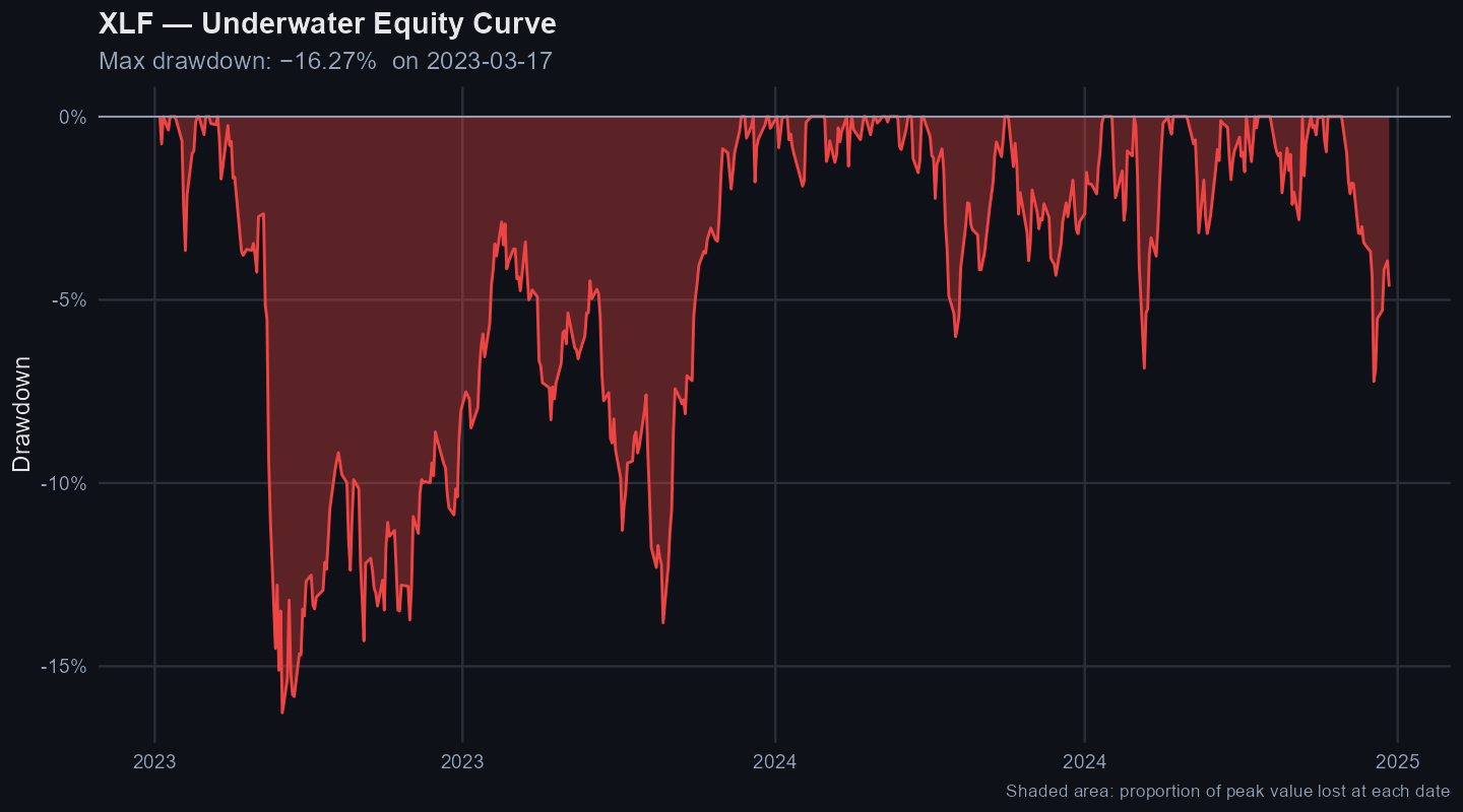
Drawdown makes the downside periods visible instead of hiding them inside one full-sample return number.
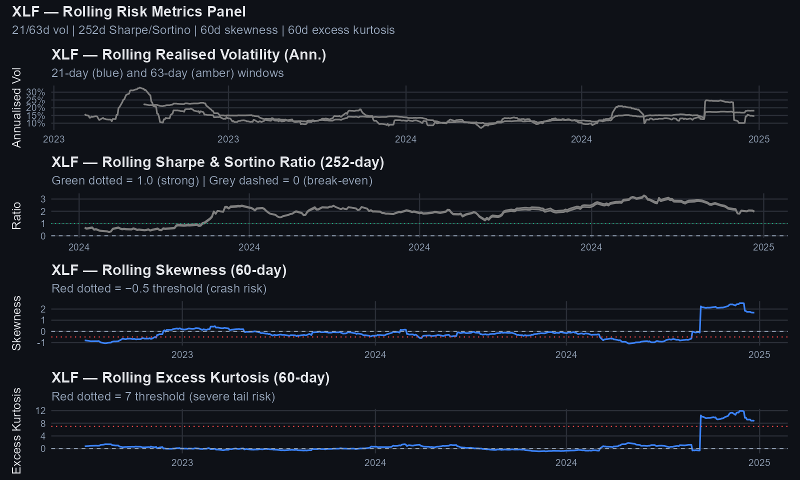
Rolling risk checks whether volatility and risk-adjusted returns were stable or clustered in specific periods.
Candidate Strategy Hypothesis
For XLF, the practical hypothesis should be conditional. A financial-sector rule may need rate, credit, or benchmark-relative context before it becomes useful, so the next design should test sector rotation and risk-controlled exposure rather than an isolated daily signal. The volatility evidence also matters: clustered variance means position sizing may be more useful than trying to forecast the next daily return.
The next tests that would add the most value are:
- Longer-horizon momentum tests, because the 2 to 16-day windows may be too short for the way many equity trends develop.
- Benchmark-relative momentum, because an asset can fail as a standalone timing trade but still matter in a pairs, sector-rotation, or relative-strength framework.
- Walk-forward rule tests with transaction costs, turnover, and cash or benchmark comparisons.
- Yield-curve-conditioned tests, because financial-sector returns can depend on the rate environment.
- Relative strength versus SPY, because sector ETFs often behave better as allocation candidates than standalone directional trades.
For automated research workflows, the resulting strategy hypothesis can be represented as:
{
  "strategy_name": "XLF Risk-Aware Allocation Test",
  "strategy_status": "hypothesis_for_backtest",
  "strategy_type": "risk_managed_allocation",
  "asset": "XLF",
  "core_thesis": "For XLF, the practical hypothesis should be conditional. A financial-sector rule may need rate, credit, or benchmark-relative context before it becomes useful, so the next design should test sector rotation and risk-controlled exposure rather than an isolated daily signal. The volatility evidence also matters: clustered variance means position sizing may be more useful than trying to forecast the next daily return.",
  "required_backtests": ["walk-forward validation", "buy-and-hold asset benchmark", "broad market benchmark", "cash or T-bill benchmark", "transaction costs", "turnover"],
  "not_investment_advice": true
}
What Would Change My Mind?
A good strategy-selection note should be falsifiable. These are the findings that would make the hypothesis stronger or force a different conclusion:
- Variance-ratio results would need to reject the random-walk benchmark at the relevant holding horizons, with p-values strong enough to survive a skeptical read.
- The mean-equation model would need to find useful structure in returns rather than selecting a flat mean process or leaving only noise in the residuals.
- A walk-forward backtest would need to beat buy-and-hold, cash or T-bills, and the relevant benchmark after transaction costs and turnover.
- Risk-managed variants would need to improve drawdown, volatility, or risk-adjusted return without simply hiding risk through lower exposure.
- For XLF, yield-curve-conditioned or SPY-relative sector tests would need to show that financial-sector exposure changes with the rate and market backdrop.
Backtested Results
The downloadable backtested results are planned for a later implementation step. They should include walk-forward results, benchmarks, turnover, and transaction-cost sensitivity before any rule is treated as validated.
Limitations
This article is a preliminary strategy-selection note for the 2023-01-03 to 2024-12-27 sample. It is useful for deciding what to test next; it is not a production trading rule.